RGErun 2: Solving Renormalization Group Equations in Effective Field Theories
A heavy particle has only indirect influence on dynamics at energies below its mass m. Several such mass thresholds mi can exist, with a different effective field theory (EFT) in each interval. At a threshold, parameters of the theories below and above it are matched. Between thresholds, the dependence of parameters such as couplings, masses, or mixing angles is described by renormalization group equations (RGEs). (For reference, see e.g. “Effective Field Theory” by Antonio Pich, or Ira Z. Rothstein’s “TASI Lectures on Effective Field Theories”.)
- RGErun 2.2.3 as a Mathematica notebook with package code and examples
- RGErun 2.2.3 as a Mathematica package
In the program, one can enter initial conditions and the RGEs in an intuitive format and easily choose which RGEs, which thresholds and matching conditions to include (it is useful for debugging). Possible degeneracy of mass thresholds is taken into account.
Vector, matrix, or tensor functions, and term-by-term multiplication of them in RGEs can be used. (As such, Mathematica allows scalar or matrix multiplication in differential equations, but not element-wise multiplication.)
How the Program Works
The run function is used to run up or down the energy scale. In the run, at first the thresholds are sorted and names of degenerate thresholds grouped together with their values. Vector, matrix, or tensor functions with right dimensions are constructed automatically according to the dimensions of their initial conditions. In each effective field theory between thresholds, the RGEs are given the list of the names of all thresholds below the current energy scale as an argument. The name of the threshold at hand can be used in the matching functions to select a right match at each threshold. At each threshold, each variable is given a new value; it can be used in matching condition. One can also use several run-ups and run-downs one after another for iteration. The solutions defined piece-wise in different intervals are put together in functions. If printOut->True, initial conditions for the couplings or variables, intermediate and matched results & parameters at each threshold are printed on the screen together with a plot of running variables.
Usage, Input Parameters & Initial Conditions
A good example is the running of the Standard Model gauge couplings at one-loop level.
- Once you have compied the package in your Mathematica library directory, you can import it with
Needs["RGErun`"]; - Enter threshold values in GeV and the names of the thresholds to use, e.g.
mt=173.34; mP=1.2*1019;Their order is not relevant: threshold values are sorted and the names of degenerate thresholds are grouped together automatically.
thresholds={"mt" -> mt, "mP" -> mP}; -
Initial conditions for functions as function definitions at some constant scale such as the mass of the top quark:
g1[mt] = Sqrt[5/3] 0.35940;

g2[mt] = 0.64754;

g3[mt] = 1.1666; -
The right hand sides of RGEs (the so-called beta functions) as
β[g1, "SM", _] := 1/(16 π2) 41/10 g13;Enter function names without arguments (such as
β[g2, "SM", _] := 1/(16 π2) (-19/6) g23;
β[g3, "SM", _] := 1/(16 π2) (-7) g33;g1, notg1[t]). The second argument toβis a string that specifies the model. The third argument stands for the thresholds of effective theories at which the RGEs can change; here the blank_indicates that we consider the Standard Model up to any energy scale. The third argument can be given a name, e.g.thresholds. UseIforWhichwithMemberQ[thresholds, "threshold name"]to check whether the threshold with"threshold name"is inthresholdsand choose between variants of the same RGE in different EFTs. To multiply a vector or matrix variable element-wise by a constant vector or matrix, use⊗. (To add a constant vector or matrix, use⊕.) Instead ofIdentityMatrix[n], use𝕀[n] (that is \[DoubleStruckCapitalI][n]). – You can also use thegetPyrateRGEsfunction to import RGEs calculated with the PyR@TE or SARAH packages. For example, read in precalculated RGEs for the two Higgs doublet model:variables = getRGEs["RGEsOutput_numerics.m", returnVariables -> True, replaceNames -> {gSU2L -> g2, gSU3c -> g3, lambda1 -> λ1, lambda2 -> λ2, lambda3 -> λ3, lambda4 -> λ4, lambda5 -> λ5, lambda6 -> λ6, lambda7 -> λ7}];IfreturnVariablesis true, thegetRGEsfunction returns the list of variables, and thereplaceNamesoption lets you to change names of the variables defined in the original PyR@TE output. -
Matching conditions and the list of matching conditions to use as
match[coupling][scale_, thresholds_, dir_] := matching condition;andmatches={variable -> match[variable], …};The name of the matching condition function could have a diffent form thanmatch[coupling](though it is a useful convention), but the argument structure has to be the same for each matching condition. Unlike for the RGEs, here the argumentthresholdsthat a matching condition will receive is the name(s) list of the current threshold.dirwill give the running direction which can be"up"or"down". Again you can useIforWhichwithMemberQ[thresholds, "threshold name"]&&uporMemberQ[thresholds, "threshold name"]&&down. Enter variable names withscaleas argument (see the second example in the notebook).Note that if you use values of other variables, the result may depend on the order of matching.
-
The variables to use as
variables={g1, g2, g3};Their beta functions will be included into the system of RGEs, they will be matched at the thresholds, if necessary, and their initial conditions and intermediate results printed out. - Optionally you can define functions of variables to print out, e.g. masses as functions of mass matrices. A simple example would be
massesE[scale_]:=v Eigenvalues[Ye[scale]];whereYeis the matrix of Yukawa couplings of leptons andvis the Higgs vacuum expectation value. The list of these functions,funs={massesE};has to be given torunas an argument. -
Finally, we are ready to run up or down: use
run[thresholds, variables, "up", "model", matches -> matches, functions  -> functions,
 printOut -> True, MaxSteps -> 106, WorkingPrecision -> MachinePrecision]
for starting at low energy and going up, or change"up"to"down"to start at some high energy and go down. Lists of possible matchings and functions to pring out at each scale can be given as options.runhas the optionprintOut(Trueby default) to print out the initial, run and matched values of variables and functions at the thresholds together with a plot of the running variables; note thatrunalso takes any options ofNDSolve. The options are used in the above example with their default values (the default ofmatchesandfunctionsis{}). After the running, the variables will be accessible as functionsvariable[μ]of the renormalisation scaleμ. Their values outside the range of running will be set to their values at the initial and final scales (and their derivatives to zero) for definiteness.
For the running of the gauge couplings, we do not have any matchings or functions, so we will simply use
run[thresholds, variables, "up", "SM", {}, {}] The result is
    ——————————————————————————————————————————————————

    RUNNING UP

    Results @ mt = 173.34 GeV

    Initial variables:

    g1 = 0.463983, g2 = 0.64754, g3 = 1.1666


    ——————————————————————————————————————————————————

    Results @ mP = 1.22 ×
         1019 GeV

    Run variables:

    g1 = 0.616534, g2 = 0.503751, g3 = 0.489476

    ——————————————————————————————————————————————————
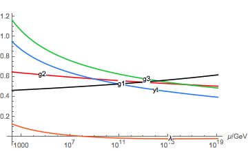
The run variables are functions of the renormalization scale μ in GeV:
g1[1000]


         0.468675
Their derivatives to all orders with respect to μ are also available:
g1'[1000]


        2.71634*10-6
The name of the model is an optional argument to the running variables:
g1[1000, "SM"]
to allow for easier comparison of different models, in which case the variable without the model name specified is given by the model that was evaluated last.
0.468675