Geometric Objects - Spatial Data Model
Overview of geometric objects - Simple Features Implementation in Shapely
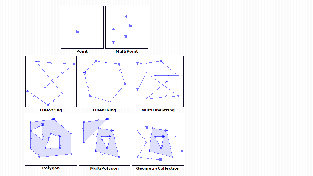
Fundamental geometric objects that can be used in Python with Shapely module
The most fundamental geometric objects are Points, Lines and Polygons which are the basic ingredients when working with spatial data in vector format. Python has a specific module called Shapely that can be used to create and work with Geometric Objects. There are many useful functionalities that you can do with Shapely such as:
Create a Line or Polygon from a Collection of Point geometries
Calculate areas/length/bounds etc. of input geometries
Make geometric operations based on the input geometries such as Union, Difference, Distance etc.
Make spatial queries between geometries such Intersects, Touches, Crosses, Within etc.
Geometric Objects consist of coordinate tuples where:
Point -object represents a single point in space. Points can be either two-dimensional (x, y) or three dimensional (x, y, z).
LineString -object (i.e. a line) represents a sequence of points joined together to form a line. Hence, a line consist of a list of at least two coordinate tuples
Polygon -object represents a filled area that consists of a list of at least three coordinate tuples that forms the outerior ring and a (possible) list of hole polygons.
It is also possible to have a collection of geometric objects (e.g. Polygons with multiple parts):
MultiPoint -object represents a collection of points and consists of a list of coordinate-tuples
MultiLineString -object represents a collection of lines and consists of a list of line-like sequences
MultiPolygon -object represents a collection of polygons that consists of a list of polygon-like sequences that construct from exterior ring and (possible) hole list tuples
Point
Creating point is easy, you pass x and y coordinates into Point() -object (+ possibly also z -coordinate) :
# Import necessary geometric objects from shapely module
In [1]: from shapely.geometry import Point, LineString, Polygon

# Create Point geometric object(s) with coordinates
In [2]: point1 = Point(2.2, 4.2)

In [3]: point2 = Point(7.2, -25.1)

In [4]: point3 = Point(9.26, -2.456)

In [5]: point3D = Point(9.26, -2.456, 0.57)

# What is the type of the point?
In [6]: point_type = type(point1)
Let’s see what the variables look like
In [7]: print(point1)
POINT (2.2 4.2)

In [8]: print(point3D)
POINT Z (9.26 -2.456 0.57)

In [9]: print(type(point1))
<class 'shapely.geometry.point.Point'>
We can see that the type of the point is shapely’s Point which is represented in a specific format that is based on the GEOS C++ library that is one of the standard libraries in GIS. GEOS, a port of the Java Topology Suite (JTS), is the geometry engine of the PostGIS spatial extension for the PostgreSQL RDBMS. The designs of JTS and GEOS are largely guided by the Open Geospatial Consortium’s Simple Features Access Specification. It runs under the hood e.g. in QGIS. 3D-points can be recognized from the capital Z -letter in front of the coordinates.
Point attributes and functions
Point -object has some built-in attributes that can be accessed and also some useful functionalities. One of the most useful ones are the ability to extract the coordinates of a Point and calculate the Euclidian distance between points.
Extracting the coordinates of a Point can be done in a couple of different ways
# Get the coordinates
In [10]: point_coords = point1.coords

# What is the type of this?
In [11]: type(point_coords)
Out[11]: shapely.coords.CoordinateSequence
Ok, we can see that the output is a Shapely CoordinateSequence. Let’s see how we can get out the actual coordinates:
# Get x and y coordinates
In [12]: xy = point_coords.xy

# Get only x coordinates of Point1
In [13]: x = point1.x

# Whatabout y coordinate?
In [14]: y = point1.y
What is inside?
In [15]: print(xy)
(array('d', [2.2]), array('d', [4.2]))

In [16]: print(x)
2.2

In [17]: print(y)
4.2
Okey, so we can see that the our xy variable contains a tuple where x and y are stored inside of a numpy arrays. However, our x and y variables are plain decimal numbers.
It is also possible to calculate the distance between points which can be useful in many applications
the returned distance is based on the projection of the points (degrees in WGS84, meters in UTM)
# Calculate the distance between point1 and point2
In [18]: point_dist = point1.distance(point2)

In [19]: print("Distance between the points is {0:.2f} decimal degrees".format(point_dist))
Distance between the points is 29.72 decimal degrees
Side note on distances in GIS
In Shapely the distance is the Euclidean Distance or Linear distance between two points on a plane. However, if we want to calculate the real distance on Earth’s surface, we need to calculate the distance on a sphere. The radius of Earth at the equator is 6378 kilometers, according to NASA’s Goddard Space Flight Center, and Earth’s polar radius is 6,356 km - a difference of 22 km. In order to approximate Earth size as a simple sphere we use these as radius. In order to calculate the distance in more human understandable values we need some math:
# law of cosines - determines the great-circle distance between two points on a sphere given their longitudes and latitudes based on "basic math"
In [20]: import math

In [21]: distance = math.acos(math.sin(math.radians(point1.y))*math.sin(math.radians(point2.y))+math.cos(math.radians(point1.y))*math.cos(math.radians(point2.y))*math.cos(math.radians(point2.x)-math.radians(point1.x)))*6378

In [22]: print( "{0:8.4f} for equatorial radius in km".format(distance))
3306.1044 for equatorial radius in km

In [23]: distance = math.acos(math.sin(math.radians(point1.y))*math.sin(math.radians(point2.y))+math.cos(math.radians(point1.y))*math.cos(math.radians(point2.y))*math.cos(math.radians(point2.x)-math.radians(point1.x)))*6356

In [24]: print( "{0:8.4f} for polar radius in km".format(distance))
3294.7004 for polar radius in km
But Earth is not a perfect sphere but an bubbly space rock (geoid). The most widely used approximations are ellipsoids. These are well-defined simplifications for computational reasons. And the most widely used standard ellipsoid is “WGS84”. So, using PyProj with the “WGS84” ellipsoid, we can easily calculate distances (and the angles towards each other, aka forward and back azimuths) between initial points (specified by lons1, lats1) and terminus points (specified by lons2, lats2).
# with pyproj
In [25]: import pyproj

In [26]: geod = pyproj.Geod(ellps='WGS84')

In [27]: angle1,angle2,distance = geod.inv(point1.x, point1.y, point2.x, point2.y)

In [28]: print ("{0:8.4f} for ellipsoid WGS84 in km".format(distance/1000))
3286.3538 for ellipsoid WGS84 in km
LineString
Creating a LineString -object is fairly similar to how Point is created. Now instead using a single coordinate-tuple we can construct the line using either a list of shapely Point -objects or pass coordinate-tuples:
# Create a LineString from our Point objects
In [29]: line = LineString([point1, point2, point3])

# It is also possible to use coordinate tuples having the same outcome
In [30]: line2 = LineString([(2.2, 4.2), (7.2, -25.1), (9.26, -2.456)])
Let’s see how our LineString looks like
In [31]: print(line)
LINESTRING (2.2 4.2, 7.2 -25.1, 9.26 -2.456)

In [32]: print(line2)
LINESTRING (2.2 4.2, 7.2 -25.1, 9.26 -2.456)

In [33]: type(line)
Out[33]: shapely.geometry.linestring.LineString
Ok, now we can see that variable line constitutes of multiple coordinate-pairs and the type of the data is shapely LineString.
LineString attributes and functions
LineString -object has many useful built-in attributes and functionalities. It is for instance possible to extract the coordinates or the length of a LineString (line), calculate the centroid of the line, create points along the line at specific distance, calculate the closest distance from a line to specified Point and simplify the geometry. See full list of functionalities from Shapely documentation. Here, we go through a few of them.
We can extract the coordinates of a LineString similarly as with Point
# Get x and y coordinates of the line
In [34]: lxy = line.xy

In [35]: print(lxy)
(array('d', [2.2, 7.2, 9.26]), array('d', [4.2, -25.1, -2.456]))
Okey, we can see that the coordinates are again stored as a numpy arrays where first array includes all x-coordinates and the second all the y-coordinates respectively.
We can extract only x or y coordinates by referring to those arrays as follows
# Extract x coordinates
In [36]: line_x = lxy[0]

# Extract y coordinates straight from the LineObject by referring to a array at index 1
In [37]: line_y = line.xy[1]

In [38]: print(line_x)
array('d', [2.2, 7.2, 9.26])

In [39]: print(line_y)
array('d', [4.2, -25.1, -2.456])
We can get specific attributes such as lenght of the line and center of the line (centroid) straight from the LineString object itself
# Get the lenght of the line
In [40]: l_length = line.length

# Get the centroid of the line
In [41]: l_centroid = line.centroid

# What type is the centroid?
In [42]: centroid_type = type(l_centroid)

# Print the outputs
In [43]: print("Length of our line: {0:.2f}".format(l_length))
Length of our line: 52.46

In [44]: print("Centroid of our line: ", l_centroid)
Centroid of our line:  POINT (6.229961354035622 -11.89241115757239)

In [45]: print("Type of the centroid:", centroid_type)
Type of the centroid: <class 'shapely.geometry.point.Point'>
Okey, so these are already fairly useful information for many different GIS tasks, and we didn’t even calculate anything yet! These attributes are built-in in every LineString object that is created. Notice that the centroid that is returned is Point -object that has its own functions as was described earlier.
Polygon
Creating a Polygon -object continues the same logic of how Point and LineString were created but Polygon object only accepts coordinate-tuples as input. Polygon needs at least three coordinate-tuples:
# Create a Polygon from the coordinates
In [46]: poly = Polygon([(2.2, 4.2), (7.2, -25.1), (9.26, -2.456)])

# We can also use our previously created Point objects (same outcome)
# --> notice that Polygon object requires x,y coordinates as input
In [47]: poly2 = Polygon([[p.x, p.y] for p in [point1, point2, point3]])

# Geometry type can be accessed as a String
In [48]: poly_type = poly.geom_type

# Using the Python's type function gives the type in a different format
In [49]: poly_type2 = type(poly)

# Let's see how our Polygon looks like
In [50]: print(poly)
POLYGON ((2.2 4.2, 7.2 -25.1, 9.26 -2.456, 2.2 4.2))

In [51]: print(poly2)
POLYGON ((2.2 4.2, 7.2 -25.1, 9.26 -2.456, 2.2 4.2))

In [52]: print("Geometry type as text:", poly_type)
Geometry type as text: Polygon

In [53]: print("Geometry how Python shows it:", poly_type2)
Geometry how Python shows it: <class 'shapely.geometry.polygon.Polygon'>
Notice that Polygon has double parentheses around the coordinates. This is because Polygon can also have holes inside of it. As the help of Polygon -object tells, a Polygon can be constructed using exterior coordinates and interior coordinates (optional) where the interior coordinates creates a hole inside the Polygon:
Help on Polygon in module shapely.geometry.polygon object:
class Polygon(shapely.geometry.base.BaseGeometry)
 |  A two-dimensional figure bounded by a linear ring
 |
 |  A polygon has a non-zero area. It may have one or more negative-space
 |  "holes" which are also bounded by linear rings. If any rings cross each
 |  other, the feature is invalid and operations on it may fail.
 |
 |  Attributes
 |  ----------
 |  exterior : LinearRing
 |      The ring which bounds the positive space of the polygon.
 |  interiors : sequence
 |      A sequence of rings which bound all existing holes.
Let’s create a Polygon with a hole inside
# Let's create a bounding box of the world and make a whole in it
# First we define our exterior
In [54]: world_exterior = [(-180, 90), (-180, -90), (180, -90), (180, 90)]

# Let's create a single big hole where we leave ten decimal degrees at the boundaries of the world
# Notice: there could be multiple holes, thus we need to provide a list of holes
In [55]: hole = [[(-170, 80), (-170, -80), (170, -80), (170, 80)]]

# World without a hole
In [56]: world = Polygon(shell=world_exterior)

# Now we can construct our Polygon with the hole inside
In [57]: world_has_a_hole = Polygon(shell=world_exterior, holes=hole)
Let’s see what we have now:
In [58]: print(world)
POLYGON ((-180 90, -180 -90, 180 -90, 180 90, -180 90))

In [59]: print(world_has_a_hole)
POLYGON ((-180 90, -180 -90, 180 -90, 180 90, -180 90), (-170 80, -170 -80, 170 -80, 170 80, -170 80))

In [60]: type(world_has_a_hole)
Out[60]: shapely.geometry.polygon.Polygon
Now we can see that the polygon has two different tuples of coordinates. The first one represents the outerior and the second one represents the hole inside of the Polygon.
Polygon attributes and functions
We can again access different attributes that are really useful such as area, centroid, bounding box, exterior, and exterior-length of the Polygon
# Get the centroid of the Polygon
In [61]: world_centroid = world.centroid

# Get the area of the Polygon
In [62]: world_area = world.area

# Get the bounds of the Polygon (i.e. bounding box)
In [63]: world_bbox = world.bounds

# Get the exterior of the Polygon
In [64]: world_ext = world.exterior

# Get the length of the exterior
In [65]: world_ext_length = world_ext.length
Let’s see what we have now
In [66]: print("Poly centroid: ", world_centroid)
Poly centroid:  POINT (-0 -0)

In [67]: print("Poly Area: ", world_area)
Poly Area:  64800.0

In [68]: print("Poly Bounding Box: ", world_bbox)
Poly Bounding Box:  (-180.0, -90.0, 180.0, 90.0)

In [69]: print("Poly Exterior: ", world_ext)
Poly Exterior:  LINEARRING (-180 90, -180 -90, 180 -90, 180 90, -180 90)

In [70]: print("Poly Exterior Length: ", world_ext_length)
Poly Exterior Length:  1080.0
Reading X/Y Coordinates from Text files
One of the “classical” problems in GIS is the situation where you have a set of coordinates in a file and you need to get them into a map (or into a GIS-software). Python is a really handy tool to solve this problem as with Python it is basically possible to read data from any kind of input datafile (such as csv-, txt-, excel-, or gpx-files (gps data) or from different databases).
Python provides various helpful packages and functions to work with data. While you could of course also manually program to open the file, read it line by line, extract fields and process variables, we can also use a widely used library called Pandas to read a file with tabular data and present it to us as a so called dataframe:
With the Windows File Explorer create a folder named L1 inside your geopython2019 working directory. Download the following file and save it into that L1 folder.
file: global-city-population-estimates.csv
In [71]: import pandas as pd

# make sure you have the correct path to your working file
# e.g. 'L1/global-city-population-estimates.csv' if you saved the file in your working directory
In [72]: df = pd.read_csv('source/_static/data/L1/global-city-population-estimates.csv', sep=';', encoding='latin1')

# this option tells pandas to print up to 20 columns, typically a the print function will cut the output for better visibility
# (depending on the size and dimension of the dataframe)
In [73]: pd.set_option('max_columns',20)

In [74]: print(df.head(5))
  Country or area Urban Agglomeration   Latitude   Longitude  Population_2015  \
0           Japan               Tokyo  35.689500  139.691710         38001018
1           India               Delhi  28.666670   77.216670         25703168
2           China            Shanghai  31.220000  121.460000         23740778
3          Brazil           S?o Paulo -23.550000  -46.640000         21066245
4           India     Mumbai (Bombay)  19.073975   72.880838         21042538

   Unnamed: 5
0         NaN
1         NaN
2         NaN
3         NaN
4         NaN
Now we want to process the tabular data. Thus, let’s see how we can go through our data and create Point -objects from them:
# we make a function, that takes a row object coming from Pandas. The single fields per row are addressed by their column name.
In [75]: def make_point(row):
   ....:     return Point(row['Longitude'], row['Latitude'])
   ....:

# Go through every row, and make a point out of its lat and lon, by **apply**ing the function from above (downwards row by row -> axis=1)
In [76]: df['points'] = df.apply(make_point, axis=1)

In [77]: print(df.head(5))
  Country or area Urban Agglomeration   Latitude   Longitude  Population_2015  \
0           Japan               Tokyo  35.689500  139.691710         38001018
1           India               Delhi  28.666670   77.216670         25703168
2           China            Shanghai  31.220000  121.460000         23740778
3          Brazil           S?o Paulo -23.550000  -46.640000         21066245
4           India     Mumbai (Bombay)  19.073975   72.880838         21042538

   Unnamed: 5                              points
0         NaN           POINT (139.69171 35.6895)
1         NaN  POINT (77.21666999999999 28.66667)
2         NaN                POINT (121.46 31.22)
3         NaN               POINT (-46.64 -23.55)
4         NaN         POINT (72.880838 19.073975)
Geometry collections (optional)
Note
This part is not obligatory but it contains some useful information related to construction and usage of geometry collections and some special geometric objects -such as bounding box.
In some occassions it is useful to store e.g. multiple lines or polygons under a single feature (i.e. a single row in a Shapefile represents more than one line or polygon object). Collections of points are implemented by using a MultiPoint -object, collections of curves by using a MultiLineString -object, and collections of surfaces by a MultiPolygon -object. These collections are not computationally significant, but are useful for modeling certain kinds of features. A Y-shaped line feature (such as road), or multiple polygons (e.g. islands on a like), can be presented nicely as a whole by a using MultiLineString or MultiPolygon accordingly. Creating and visualizing a minimum bounding box e.g. around your data points is a really useful function for many purposes (e.g. trying to understand the extent of your data), here we demonstrate how to create one using Shapely.
Geometry collections can be constructed in a following manner:
# Import collections of geometric objects + bounding box
In [78]: from shapely.geometry import MultiPoint, MultiLineString, MultiPolygon, box

# Create a MultiPoint object of our points 1,2 and 3
In [79]: multi_point = MultiPoint([point1, point2, point3])

# It is also possible to pass coordinate tuples inside
In [80]: multi_point2 = MultiPoint([(2.2, 4.2), (7.2, -25.1), (9.26, -2.456)])

# We can also create a MultiLineString with two lines
In [81]: line1 = LineString([point1, point2])

In [82]: line2 = LineString([point2, point3])

In [83]: multi_line = MultiLineString([line1, line2])

# MultiPolygon can be done in a similar manner
# Let's divide our world into western and eastern hemispheres with a hole on the western hemisphere
# --------------------------------------------------------------------------------------------------
# Let's create the exterior of the western part of the world
In [84]: west_exterior = [(-180, 90), (-180, -90), (0, -90), (0, 90)]

# Let's create a hole --> remember there can be multiple holes, thus we need to have a list of hole(s).
# Here we have just one.
In [85]: west_hole = [[(-170, 80), (-170, -80), (-10, -80), (-10, 80)]]

# Create the Polygon
In [86]: west_poly = Polygon(shell=west_exterior, holes=west_hole)

# Let's create the Polygon of our Eastern hemisphere polygon using bounding box
# For bounding box we need to specify the lower-left corner coordinates and upper-right coordinates
In [87]: min_x, min_y = 0, -90

In [88]: max_x, max_y = 180, 90

# Create the polygon using box() function
In [89]: east_poly_box = box(minx=min_x, miny=min_y, maxx=max_x, maxy=max_y)

# Let's create our MultiPolygon. We can pass multiple Polygon -objects into our MultiPolygon as a list
In [90]: multi_poly = MultiPolygon([west_poly, east_poly_box])
Let’s see what do we have:
In [91]: print("MultiPoint:", multi_point)
MultiPoint: MULTIPOINT (2.2 4.2, 7.2 -25.1, 9.26 -2.456)

In [92]: print("MultiLine: ", multi_line)
MultiLine:  MULTILINESTRING ((2.2 4.2, 7.2 -25.1), (7.2 -25.1, 9.26 -2.456))

In [93]: print("Bounding box: ", east_poly_box)
Bounding box:  POLYGON ((180 -90, 180 90, 0 90, 0 -90, 180 -90))

In [94]: print("MultiPoly: ", multi_poly)
MultiPoly:  MULTIPOLYGON (((-180 90, -180 -90, 0 -90, 0 90, -180 90), (-170 80, -170 -80, -10 -80, -10 80, -170 80)), ((180 -90, 180 90, 0 90, 0 -90, 180 -90)))
We can see that the outputs are similar to the basic geometric objects that we created previously but now these objects contain multiple features of those points, lines or polygons.
Geometry collection -objects’ attributes and functions
We can also get many useful attributes from those objects:
# Convex Hull of our MultiPoint --> https://en.wikipedia.org/wiki/Convex_hull
In [95]: convex = multi_point.convex_hull

# How many lines do we have inside our MultiLineString?
In [96]: lines_count = len(multi_line)

# Let's calculate the area of our MultiPolygon
In [97]: multi_poly_area = multi_poly.area

# We can also access different items inside our geometry collections. We can e.g. access a single polygon from
# our MultiPolygon -object by referring to the index
# Let's calculate the area of our Western hemisphere (with a hole) which is at index 0
In [98]: west_area = multi_poly[0].area

# We can check if we have a "valid" MultiPolygon. MultiPolygon is thought as valid if the individual polygons
# does notintersect with each other. Here, because the polygons have a common 0-meridian, we should NOT have
# a valid polygon. This can be really useful information when trying to find topological errors from your data
In [99]: valid = multi_poly.is_valid
Let’s see what do we have:
In [100]: print("Convex hull of the points: ", convex)
Convex hull of the points:  POLYGON ((7.2 -25.1, 2.2 4.2, 9.26 -2.456, 7.2 -25.1))

In [101]: print("Number of lines in MultiLineString:", lines_count)
Number of lines in MultiLineString: 2

In [102]: print("Area of our MultiPolygon:", multi_poly_area)
Area of our MultiPolygon: 39200.0

In [103]: print("Area of our Western Hemisphere polygon:", west_area)
Area of our Western Hemisphere polygon: 6800.0

In [104]: print("Is polygon valid?: ", valid)
Is polygon valid?:  False
From the above we can see that MultiPolygons have exactly the same attributes available as single geometric objects but now the information such as area calculates the area of ALL of the individual -objects combined. There are also some extra features available such as is_valid attribute that tells if the polygons or lines intersect with each other.
Launch in the web/MyBinder:
Acknowledgments:
These materials are partly based on Shapely -documentation and Westra E. (2016), Chapter 3.