Coordinate Reference Systems (CRS)
Coordinate reference systems (CRS) are important because the geometric shapes in a GeoDataFrame are simply a collection of coordinates in an arbitrary space. A CRS tells Python how those coordinates related to places on the Earth. A map projection (or a projected coordinate system) is a systematic transformation of the latitudes and longitudes into a plain surface where units are quite commonly represented as meters (instead of decimal degrees).
As map projections of gis-layers are fairly often defined differently (i.e. they do not match), it is a common procedure to redefine the map projections to be identical in both layers. It is important that the layers have the same projection as it makes it possible to analyze the spatial relationships between layers, such as in conducting the Point in Polygon spatial query.
Coordinate Reference Systems (CRS), also referred to as Spatial Reference Systems (SRS), include two common types:
Geographic Coordinate Sytems
Projected Coordinate Systems
Attention
In developer jargon and often also sloppily used by GIS technicians, the term “projection” is often used for all types of CRS/SRS. For example, WGS84 is called WGS84 projection. To be correct, WGS84, is a Geographic Coordinate System and NOT a projection.
Geographic coordinate system (GCS)
A geographic coordinate system uses a ellipsoidal surface to define locations on the Earth. There are three parts to a geographic coordinate system:
A datum - an ellipsoidal (spheroid) model of the Earth to use. Common datums include WGS84 (used in GPS).
A prime meridian
Angular unit of measure
Both latitude and longitude are typically represented in two ways:
Degrees, Minutes, Seconds (DMS), for example, 58° 23′ 12′ ′N, 26° 43′ 21′ ′E
Decimal Degrees (DD) used by computers and stored as float data type, for example, 58.38667 and 26.7225
Projected coordinate system (PCS)
Projected coordinate systems define a flat 2D Cartesian surface. Unlike a geographic coordinate system, a projected coordinate system has constant lengths, angles, and areas across the two dimensions. A projected coordinate system is always based on a geographic coordinate system that references a specific datum.
Projected Coordinate Systems consist of:
Geographic Coordinate System
Projection Method
Projection Parameters (standard points and lines, Latitude of Origin, Longitude of Origin, False Easting, False Northing etc)
Linear units (meters, kilometers, miles etc)
Defining and changing CRSs in Geopandas
Luckily, defining and changing CRSs is easy in Geopandas. In this tutorial we will see how to retrieve the coordinate reference system information from the data, and how to change it. We will re-project a data file from WGS84 (lat, lon coordinates) into a Lambert Azimuthal Equal Area projection which is the recommended projection for Europe by European Commission.
Note
Choosing an appropriate projection for your map is not always straightforward because it depends on what you actually want to represent with your map, and what is the spatial scale of your data. In fact, there does not exist a “perfect projection” since each one of them has some strengths and weaknesses, and you should choose such projection that fits best for your needs. You can read more about how to choose a map projection from here, and a nice blog post about the strengths and weaknesses of few commonly used projections.
Download data
For this tutorial we will be using a Shapefile representing Europe. Download and extract Europe_borders.zip file that contains a Shapefile with following files:
Europe_borders.cpg  Europe_borders.prj  Europe_borders.sbx  Europe_borders.shx
Europe_borders.dbf  Europe_borders.sbn  Europe_borders.shp
Changing Coordinate Reference System
GeoDataFrame that is read from a Shapefile contains always (well not always but should) information about the coordinate system in which the data is projected.
Let’s start by reading the data from the Europe_borders.shp file.
In [1]: import geopandas as gpd

# Filepath to the Europe borders Shapefile
In [2]: fp = "source/_static/data/L2/Europe_borders.shp"

# Read data
In [3]: data = gpd.read_file(fp)
We can see the current coordinate reference system from .crs
attribute:
In [4]: data.crs
Out[4]:
<Geographic 2D CRS: EPSG:4326>
Name: WGS 84
Axis Info [ellipsoidal]:
- Lat[north]: Geodetic latitude (degree)
- Lon[east]: Geodetic longitude (degree)
Area of Use:
- name: World
- bounds: (-180.0, -90.0, 180.0, 90.0)
Datum: World Geodetic System 1984
- Ellipsoid: WGS 84
- Prime Meridian: Greenwich
So from this disctionary we can see that the data is something called epsg:4326. The EPSG number (“European Petroleum Survey Group”) is a code that tells about the coordinate system of the dataset. “EPSG Geodetic Parameter Dataset is a collection of definitions of coordinate reference systems and coordinate transformations which may be global, regional, national or local in application”. EPSG-number 4326 that we have here belongs to the WGS84 coordinate system (i.e. coordinates are in decimal degrees (lat, lon)).
You can find a lot of information about different available coordinate reference systems from:
Let’s also check the values in our geometry column.
In [5]: data['geometry'].head()
Out[5]:
0    MULTIPOLYGON (((19.50115 40.96230, 19.50563 40...
1    POLYGON ((1.43992 42.60649, 1.45041 42.60596, ...
2    POLYGON ((16.00000 48.77775, 16.00000 48.78252...
3    POLYGON ((5.00000 49.79374, 4.99724 49.79696, ...
4    POLYGON ((19.22947 43.53458, 19.22925 43.53597...
Name: geometry, dtype: geometry
So the coordinate values of the Polygons indeed look like lat-lon values.
Let’s convert (aka reproject) those geometries into Lambert Azimuthal Equal Area projection (EPSG: 3035).
Changing the CRS is really easy to do in Geopandas
with .to_crs() -function. As an input for the function, you
should define the epgs value of the target CRS that you want to use.
# Let's take a copy of our layer
In [6]: data_proj = data.copy()

# Reproject the geometries by replacing the values with projected ones
In [7]: data_proj = data_proj.to_crs(epsg=3035)
Let’s see how the coordinates look now.
In [8]: data_proj['geometry'].head()
Out[8]:
0    MULTIPOLYGON (((5122010.375 2035145.186, 51223...
1    POLYGON ((3618045.758 2206753.801, 3618896.570...
2    POLYGON ((4761568.782 2869552.349, 4761526.557...
3    POLYGON ((3961258.262 2976824.238, 3961083.984...
4    POLYGON ((5066801.274 2315488.073, 5066765.564...
Name: geometry, dtype: geometry
And here we go, the numbers have changed! Now we have successfully changed the CRS of our layer into a new one, i.e. to ETRS-LAEA projection.
Note
There is also possibility to pass the CRS information as proj4 strings or dictionaries, see more here
To really understand what is going on, it is good to explore our data visually. Hence, let’s compare the datasets by making maps out of them.
import matplotlib.pyplot as plt

%matplotlib inline

# Plot the WGS84
data.plot(facecolor='gray');

# Add title
plt.title("WGS84 CRS");

# Remove empty white space around the plot
plt.tight_layout()

# Plot the one with ETRS-LAEA projection
data_proj.plot(facecolor='blue');

# Add title
plt.title("ETRS Lambert Azimuthal Equal Area projection");

# Remove empty white space around the plot
plt.tight_layout()
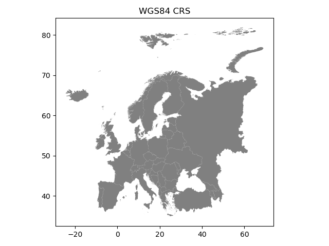
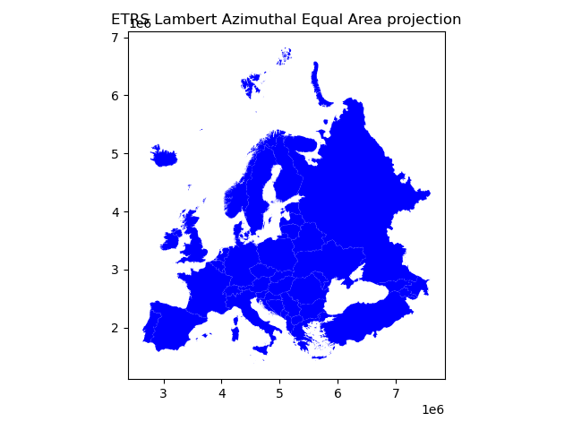
Indeed, they look quite different and our re-projected one looks much better in Europe as the areas especially in the north are more realistic and not so stretched as in WGS84.
Finally, let’s save our projected layer into a Shapefile so that we can use it later.
# Ouput file path
out_fp = "Europe_borders_epsg3035.shp"

# Save to disk
data_proj.to_file(out_fp)
Note
It is possible to pass more specific coordinate reference definition information as proj4 text, like following example for EPSG:3035
data_proj.crs = '+proj=laea +lat_0=52 +lon_0=10 +x_0=4321000 +y_0=3210000 +ellps=GRS80 +units=m +no_defs'
You can find proj4 text versions for different CRS from spatialreference.org or
http://epsg.io/. Each page showing spatial reference information has links for different formats for the CRS.
Click a link that says Proj4 and you will get the correct proj4 text presentation for your CRS.
Calculating distances
Let’s, continue working with our Europe_borders.shp file and find out the Euclidean distances from
the centroids of the European countries to Tartu, Estonia. We will calculate the distance between Tartu and
other European countries (centroids) using a metric projection (World Azimuthal Equidistant) that gives us the distance
in meters.
Let’s first import necessary packages.
In [9]: from shapely.geometry import Point

In [10]: from fiona.crs import from_epsg
Next we need to specify our CRS to metric system using World Azimuthal Equidistant -projection where distances are represented correctly from the center point.
Let’s specify our target location to be the coordinates of Tartu (lon=26.7290 and lat=58.3780).
In [11]: tartu_lon = 26.7290

In [12]: tartu_lat = 58.3780
Next we need to specify a Proj4 string to reproject our data into World Azimuthal Equidistant
in which we also want to center our projection to Tartu. We need to specify the +lat_0 and +lon_0 parameters in Proj4 string to do this.
In [13]: proj4_txt = '+proj=aeqd +lat_0=58.3780 +lon_0=26.7290 +x_0=0 +y_0=0 +ellps=WGS84 +datum=WGS84 +units=m +no_defs'
Now we are ready to transform our Europe_borders.shp data into the desired projection. Let’s create a new
copy of our GeoDataFrame called data_d (d for ‘distance’).
In [14]: data_d = data.to_crs(proj4_txt)
Let’s take a look of our data and create a map, so we can see what we have now.
In [15]: data_d.plot(facecolor='purple');

In [16]: plt.title("World Azimuthal Equidistant, centred on Tartu");

In [17]: plt.tight_layout();
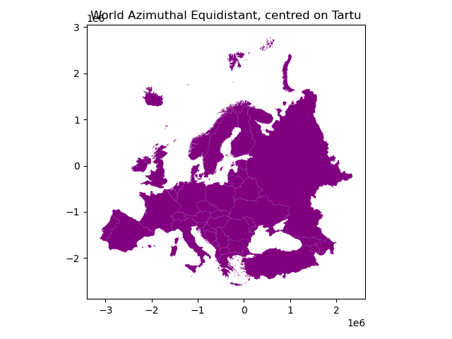
From here we can see that indeed our map is now centered to Tartu as the 0-position in both x and y is on top of Tartu.
Let’s continue our analysis by creating a Point object from Tartu and insert it into a GeoPandas GeoSeries. We also specify that the CRS of the GeoSeries is WGS84. You can do this by using
crsparameter when creating the GeoSeries.
In [18]: tartu = gpd.GeoSeries([Point(tartu_lon, tartu_lat)], crs=from_epsg(4326))
Let’s convert this point to the same CRS as our Europe data is.
In [19]: tartu = tartu.to_crs(proj4_txt)

In [20]: print(tartu)
0    POINT (0.00000 0.00000)
dtype: geometry
Aha! So the Point coordinates of Tartu are 0. This confirms us that the center point of our projection is indeed Tartu.
Next we need to calculate the centroids for all the Polygons of the European countries. This can be done easily in Geopandas by using the centroid attribute.
In [21]: data_d['country_centroid'] = data_d.centroid

In [22]: data_d.head(2)
Out[22]:
      NAME  ORGN_NAME                                           geometry  \
0  Albania  Shqipëria  MULTIPOLYGON (((-616930.849 -1905901.378, -616...
1  Andorra    Andorra  POLYGON ((-2059909.806 -1383253.286, -2059109....

                    country_centroid
0   POINT (-566125.440 -1891201.934)
1  POINT (-2051296.405 -1393144.787)
So now we have a new column country_centroid that has the Point geometries representing the centroids of each Polygon.
Now we can calculate the distances between the centroids and Tartu.
We saw an example in an erarlier lesson/exercise where we used apply() function for doing the loop instead of using the iterrows() function.
In (Geo)Pandas, the apply() function takes advantage of numpy when looping, and is hence much faster
which can give a lot of speed benefit when you have many rows to iterate over. Here, we will see how we can use that
to calculate the distance between the centroids and Tartu. We will create our own function to do this calculation.
Let’s first create our function called
calculateDistance().
def def calculateDistance(row, dest_geom, src_col='geometry'):
    """
    Calculates the distance between a single Shapely Point geometry and a GeoDataFrame with Point geometries.

    Parameters
    ----------
    dest_geom : shapely.Point
        A single Shapely Point geometry to which the distances will be calculated to.
    src_col : str
        A name of the column that has the Shapely Point objects from where the distances will be calculated from.
    """
    # Calculate the distances
    dist = row[src_col].distance(dest_geom)
    # Tranform into kilometers
    dist_km = dist/1000
    # return the distance value
    return dist_km
The parameter row is used to pass the data from each row of our GeoDataFrame into our function and then the other paramaters are used for passing other necessary information for using our function.
Before using our function and calculating the distances between Tartu and centroids, we need to get the Shapely point geometry from the re-projected Tartu center point. We can use the
get()function to retrieve a value from specific index (here index 0).
In [23]: tartu_geom = tartu.get(0)

In [24]: print(tartu_geom)
POINT (0 0)
Now we are ready to use our function with apply() function. When using the function, it is important to specify that the axis=1.
This specifies that the calculations should be done row by row (instead of column-wise).
In [25]: data_d['dist_to_tartu'] = data_d.apply(calculateDistance, dest_geom=tartu_geom, src_col='country_centroid', axis=1)

In [26]: data_d.head(20)
Out[26]:
                  NAME            ORGN_NAME  \
0              Albania            Shqipëria
1              Andorra              Andorra
2              Austria           Österreich
3              Belgium    België / Belgique
4   Bosnia Herzegovina  Bosna i Hercegovina
5              Croatia             Hrvatska
6       Czech Republic                Cesko
7              Denmark              Danmark
8              Estonia                Eesti
9              Finland                Suomi
10              France               France
11             Germany          Deutschland
12      Gibraltar (UK)       Gibraltar (UK)
13              Greece               Elláda
14             Hungary         Magyarország
15             Ireland       Éire / Ireland
16               Italy               Italia
17              Latvia              Latvija
18       Liechtenstein        Liechtenstein
19           Lithuania              Lietuva

                                             geometry  \
0   MULTIPOLYGON (((-616930.849 -1905901.378, -616...
1   POLYGON ((-2059909.806 -1383253.286, -2059109....
2   POLYGON ((-789218.354 -1007540.792, -789139.78...
3   POLYGON ((-1545487.015 -710685.915, -1545569.4...
4   POLYGON ((-611931.236 -1618946.307, -611934.02...
5   MULTIPOLYGON (((-993254.065 -1456331.349, -994...
6   POLYGON ((-836233.081 -763077.620, -835498.235...
7   MULTIPOLYGON (((-937254.738 -280819.978, -9379...
8   MULTIPOLYGON (((-162360.830 -27988.570, -16287...
9   MULTIPOLYGON (((-257841.948 215108.641, -25828...
10  MULTIPOLYGON (((-2173602.950 -842389.063, -217...
11  MULTIPOLYGON (((-875698.584 -338558.972, -8751...
12  POLYGON ((-2872328.164 -1823613.920, -2871222....
13  MULTIPOLYGON (((-179277.557 -2308324.469, -179...
14  POLYGON ((-327631.708 -1104374.898, -328196.45...
15  MULTIPOLYGON (((-2437224.463 -61584.487, -2437...
16  MULTIPOLYGON (((-1274682.411 -2153336.082, -12...
17  POLYGON ((-273271.541 -72773.912, -271581.262 ...
18  POLYGON ((-1296487.801 -1075491.781, -1295313....
19  MULTIPOLYGON (((-32572.279 -376032.729, -32792...

                     country_centroid  dist_to_tartu
0    POINT (-566125.440 -1891201.934)    1974.118225
1   POINT (-2051296.405 -1393144.787)    2479.651052
2    POINT (-948755.523 -1114052.808)    1463.301302
3    POINT (-1539443.737 -612758.131)    1656.912655
4    POINT (-720901.335 -1534770.531)    1695.647168
5    POINT (-817203.750 -1426447.263)    1643.950658
6     POINT (-820305.756 -893458.815)    1212.918046
7    POINT (-1031556.205 -139241.433)    1040.911322
8        POINT (-68261.667 33616.470)      76.090225
9       POINT (-27931.560 653427.451)     654.024163
10  POINT (-1831378.471 -1000651.990)    2086.923935
11   POINT (-1139442.791 -679758.159)    1326.801051
12  POINT (-2872770.961 -1826002.350)    3403.982605
13   POINT (-328899.332 -2144633.146)    2169.706455
14   POINT (-558238.872 -1217994.425)    1339.828742
15      POINT (-2237106.677 7215.406)    2237.118313
16  POINT (-1195556.668 -1620794.614)    2014.033498
17    POINT (-109175.095 -167263.043)     199.740149
18  POINT (-1298486.108 -1089777.446)    1695.193516
19    POINT (-178650.961 -335302.276)     379.926022
Great! Now we have successfully calculated the distances between the Polygon centroids and Tartu. :)
Let’s check what is the longest and mean distance to Tartu from the centroids of other European countries.
In [27]: max_dist = data_d['dist_to_tartu'].max()

In [28]: mean_dist = data_d['dist_to_tartu'].mean()

In [29]: print("Maximum distance to Tartu is {:.2f} km, and the mean distance is {:.2f} km.".format(max_dist, mean_dist))
Maximum distance to Tartu is 3403.98 km, and the mean distance is 1688.60 km.
Note
If you would like to calculate distances between multiple locations across the globe, it is recommended to use Haversine formula to do the calculations. Haversine package in Python provides an easy-to-use function for calculating these based on latitude and longitude values.
Launch in the web/MyBinder: