Introduction to Geopandas¶

Downloading data¶

For this lesson we are using data that you can download from here. Once you have downloaded the damselfish-data.zip file into your geopython2019 directory (ideally under L2), you can unzip the file using e.g. 7Zip (on Windows).

DAMSELFISH_distributions.dbf   DAMSELFISH_distributions.prj
DAMSELFISH_distributions.sbn   DAMSELFISH_distributions.sbx
DAMSELFISH_distributions.shp   DAMSELFISH_distributions.shp.xml
DAMSELFISH_distributions.shx

The data includes a Shapefile called DAMSELFISH_distribution.shp (and files related to it).

Reading a Shapefile¶

Spatial data can be read easily with geopandas using gpd.from_file() -function:

# Import necessary module
In [1]: import geopandas as gpd

# Set filepath relative to your ``geopython2019`` working directory, from where your Jupyter Notebook or spyder also should be started
In [2]: fp = "source/_static/data/L2/DAMSELFISH_distributions.shp"

# depending if you have your notebook file (.ipynb) also under L1
# fp = "DAMSELFISH_distributions.shp"
# or full path for Windows with "r" and "\" backslashes
# fp = r"C:\Users\Alex\geopython2019\L2\DAMSELFISH_distributions.shp"
# Read file using gpd.read_file()
In [3]: data = gpd.read_file(fp)

Let’s see what datatype is our ‘data’ variable

In [4]: type(data)
Out[4]: geopandas.geodataframe.GeoDataFrame

So from the above we can see that our data -variable is a GeoDataFrame. GeoDataFrame extends the functionalities of pandas.DataFrame in a way that it is possible to use and handle spatial data within pandas (hence the name geopandas). GeoDataFrame have some special features and functions that are useful in GIS.

Let’s take a look at our data and print the first 5 rows using the head() -function prints the first 5 rows by default

In [5]: data.head()
Out[5]: 
      ID_NO             BINOMIAL  ORIGIN COMPILER  YEAR  \
183963.0   Stegastes leucorus       1     IUCN  2010   
183963.0   Stegastes leucorus       1     IUCN  2010   
183963.0   Stegastes leucorus       1     IUCN  2010   
183793.0  Chromis intercrusma       1     IUCN  2010   
183793.0  Chromis intercrusma       1     IUCN  2010   

                                            CITATION SOURCE DIST_COMM ISLAND  \
International Union for Conservation of Nature...   None      None   None   
International Union for Conservation of Nature...   None      None   None   
International Union for Conservation of Nature...   None      None   None   
International Union for Conservation of Nature...   None      None   None   
International Union for Conservation of Nature...   None      None   None   

  SUBSPECIES  ... RL_UPDATE KINGDOM_NA  PHYLUM_NAM      CLASS_NAME  \
     None  ...    2012.1   ANIMALIA    CHORDATA  ACTINOPTERYGII   
     None  ...    2012.1   ANIMALIA    CHORDATA  ACTINOPTERYGII   
     None  ...    2012.1   ANIMALIA    CHORDATA  ACTINOPTERYGII   
     None  ...    2012.1   ANIMALIA    CHORDATA  ACTINOPTERYGII   
     None  ...    2012.1   ANIMALIA    CHORDATA  ACTINOPTERYGII   

    ORDER_NAME     FAMILY_NAM GENUS_NAME   SPECIES_NA CATEGORY  \
PERCIFORMES  POMACENTRIDAE  Stegastes     leucorus       VU   
PERCIFORMES  POMACENTRIDAE  Stegastes     leucorus       VU   
PERCIFORMES  POMACENTRIDAE  Stegastes     leucorus       VU   
PERCIFORMES  POMACENTRIDAE    Chromis  intercrusma       LC   
PERCIFORMES  POMACENTRIDAE    Chromis  intercrusma       LC   

                                            geometry  
POLYGON ((-115.64375 29.71392, -115.61585 29.6...  
POLYGON ((-105.58995 21.89340, -105.56483 21.8...  
POLYGON ((-111.15962 19.01536, -111.15948 18.9...  
POLYGON ((-80.86500 -0.77894, -80.75930 -0.833...  
POLYGON ((-67.33922 -55.67610, -67.33755 -55.6...  

[5 rows x 24 columns]

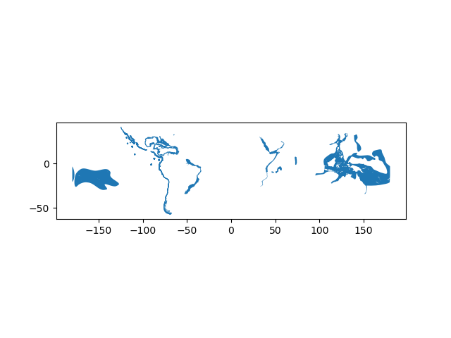
Let’s also take a look how our data looks like on a map. If you just want to explore your data on a map, you can use .plot() -function in geopandas that creates a simple map out of the data (uses matplotlib as a backend):

# import matplotlib and make it show plots directly (inline) in Jupyter notebooks
import matplotlib.pyplot as plt
%matplotlib inline

In [6]: data.plot()
Out[6]: <AxesSubplot:>

Writing a Shapefile¶

Writing a new Shapefile is also something that is needed frequently.

Let’s select 50 first rows of the input data and write those into a new Shapefile by first selecting the data using index slicing and then write the selection into a Shapefile with the gpd.to_file() -function:

# Create a output path for the data
out_file_path = r"Data\DAMSELFISH_distributions_SELECTION.shp"

# Select first 50 rows, this a the numpy/pandas syntax to ``slice`` parts out a dataframe or array, from position 0 until (excluding) 50
selection = data[0:50]

# Write those rows into a new Shapefile (the default output file format is Shapefile)
selection.to_file(out_file_path)

Task: Open the Shapefile now in QGIS (or ArcGIS) on your computer, and see how the data looks like.

Geometries in Geopandas¶

Geopandas takes advantage of Shapely’s geometric objects. Geometries are typically stored in a column called geometry (or geom). This is a default column name for storing geometric information in geopandas.

Let’s print the first 5 rows of the column ‘geometry’:

# It is possible to use only specific columns by specifying the column name within square brackets []
In [7]: data['geometry'].head()
Out[7]: 
0    POLYGON ((-115.64375 29.71392, -115.61585 29.6...
1    POLYGON ((-105.58995 21.89340, -105.56483 21.8...
2    POLYGON ((-111.15962 19.01536, -111.15948 18.9...
3    POLYGON ((-80.86500 -0.77894, -80.75930 -0.833...
4    POLYGON ((-67.33922 -55.67610, -67.33755 -55.6...
Name: geometry, dtype: geometry

Since spatial data is stored as Shapely objects, it is possible to use all of the functionalities of Shapely module that we practiced earlier.

Let’s print the areas of the first 5 polygons:

# Make a selection that contains only the first five rows
In [8]: selection = data[0:5]

We can iterate over the selected rows using a specific .iterrows() -function in (geo)pandas and print the area for each polygon:

In [9]: for index, row in selection.iterrows():
   ...:     poly_area = row['geometry'].area
   ...:     print("Polygon area at index {0} is: {1:.3f}".format(index, poly_area))
   ...: 
Polygon area at index 0 is: 19.396
Polygon area at index 1 is: 6.146
Polygon area at index 2 is: 2.697
Polygon area at index 3 is: 87.461
Polygon area at index 4 is: 0.001

Hence, as you might guess from here, all the functionalities of Pandas are available directly in Geopandas without the need to call pandas separately because Geopandas is an extension for Pandas.

Let’s next create a new column into our GeoDataFrame where we calculate and store the areas individual polygons. Calculating the areas of polygons is really easy in geopandas by using GeoDataFrame.area attribute:

In [10]: data['area'] = data.area

Let’s see the first 2 rows of our ‘area’ column.

In [11]: data['area'].head(2)
Out[11]: 
0    19.396254
1     6.145902
Name: area, dtype: float64

So we can see that the area of our first polygon seems to be 19.39 and 6.14 for the second polygon. They correspond to the ones we saw in previous step when iterating rows, hence, everything seems to work as it should. Let’s check what is the min and the max of those areas using familiar functions from our previous Pandas lessions.

# Maximum area
In [12]: max_area = data['area'].max()

# Mean area
In [13]: mean_area = data['area'].mean()

In [14]: print("Max area: {:.2f}\nMean area: {:.2f}".format(round(max_area, 2), round(mean_area, 2)))
Max area: 1493.20
Mean area: 19.96

So the largest Polygon in our dataset seems to be 1494 square decimal degrees (~ 165 000 km2) and the average size is ~20 square decimal degrees (~2200 km2).

Creating geometries into a GeoDataFrame¶

Since geopandas takes advantage of Shapely geometric objects it is possible to create a Shapefile from a scratch by passing Shapely’s geometric objects into the GeoDataFrame. This is useful as it makes it easy to convert e.g. a text file that contains coordinates into a Shapefile.

Let’s create an empty GeoDataFrame.

# Import necessary modules first
import pandas as pd
import geopandas as gpd
from shapely.geometry import Point, Polygon
import fiona

# Create an empty geopandas GeoDataFrame
newdata = gpd.GeoDataFrame()

# Let's see what's inside
In [15]: newdata
Out[15]: 
Empty GeoDataFrame
Columns: []
Index: []

The GeoDataFrame is empty since we haven’t placed any data inside.

Let’s create a new column called geometry that will contain our Shapely objects:

# Create a new column called 'geometry' to the GeoDataFrame
In [16]: newdata['geometry'] = None

# Let's see what's inside
In [17]: newdata
Out[17]: 
Empty GeoDataFrame
Columns: [geometry]
Index: []

Now we have a geometry column in our GeoDataFrame but we don’t have any data yet.

Let’s create a Shapely Polygon representing the Tartu Townhall square that we can insert to our GeoDataFrame:

# Coordinates of the Tartu Townhall square in Decimal Degrees
In [18]: coordinates = [(26.722117, 58.380184), (26.724853, 58.380676), (26.724961, 58.380518), (26.722372, 58.379933)]

# Create a Shapely polygon from the coordinate-tuple list
In [19]: poly = Polygon(coordinates)

# Let's see what we have
In [20]: poly
Out[20]: <shapely.geometry.polygon.Polygon at 0x2a4d87ddb48>

So now we have appropriate Polygon -object.

Let’s insert the polygon into our ‘geometry’ column in our GeoDataFrame:

# Insert the polygon into 'geometry' -column at index 0
In [21]: newdata.loc[0, 'geometry'] = poly

# Let's see what we have now
In [22]: newdata
Out[22]: 
                                            geometry
0  POLYGON ((26.72212 58.38018, 26.72485 58.38068...

Now we have a GeoDataFrame with Polygon that we can export to a Shapefile.

Let’s add another column to our GeoDataFrame called Location with the text Tartu Townhall Square.

# Add a new column and insert data
In [23]: newdata.loc[0, 'Location'] = 'Tartu Townhall Square'

# Let's check the data
In [24]: newdata
Out[24]: 
                                            geometry               Location
0  POLYGON ((26.72212 58.38018, 26.72485 58.38068...  Tartu Townhall Square

Now we have additional information that is useful to be able to recognize what the feature represents.

Before exporting the data it is useful to determine the coordinate reference system (projection) for the GeoDataFrame.

GeoDataFrame has a property called .crs that (more about projection on next tutorial) shows the coordinate system of the data which is empty (None) in our case since we are creating the data from the scratch:

In [25]: print(newdata.crs)
None

Let’s add a crs for our GeoDataFrame. A Python module called fiona has a nice function called from_epsg() for passing coordinate system for the GeoDataFrame. Next we will use that and determine the projection to WGS84 (epsg code: 4326):

 # Import specific function 'from_epsg' from fiona module
In [26]: from fiona.crs import from_epsg

 # Set the GeoDataFrame's coordinate system to WGS84
In [27]: newdata.crs = from_epsg(4326)

 # Let's see how the crs definition looks like
In [28]: newdata.crs
Out[28]: 
<Geographic 2D CRS: +init=epsg:4326 +no_defs +type=crs>
Name: WGS 84
Axis Info [ellipsoidal]:
- lon[east]: Longitude (degree)
- lat[north]: Latitude (degree)
Area of Use:
- name: World
- bounds: (-180.0, -90.0, 180.0, 90.0)
Datum: World Geodetic System 1984
- Ellipsoid: WGS 84
- Prime Meridian: Greenwich

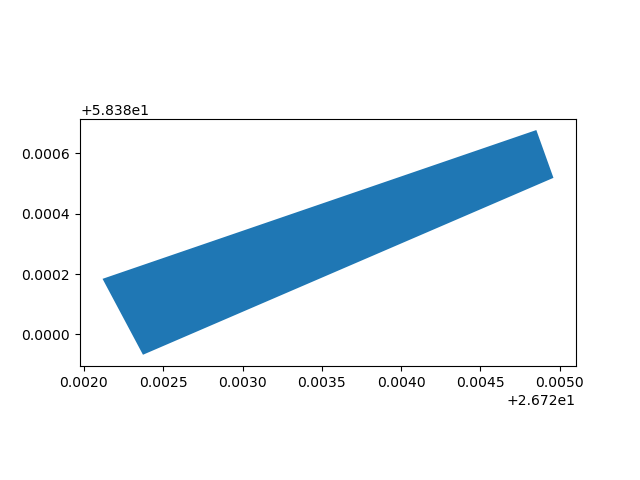
In [29]: newdata.plot()
Out[29]: <AxesSubplot:>

Finally, we can export the data using GeoDataFrames .to_file() -function. The function works similarly as numpy or pandas, but here we only need to provide the output path for the Shapefile:

# Determine the output path for the Shapefile
out_file = "raekoja_plats.shp"

# Write the data into that Shapefile
newdata.to_file(out_file)

Now we have successfully created a Shapefile from the scratch using only Python programming. Similar approach can be used to for example to read coordinates from a text file (e.g. points) and create Shapefiles from those automatically.

Task: check the output Shapefile in QGIS and make sure that the attribute table seems correct.

Practical example: Save multiple Shapefiles¶

One really useful function that can be used in Pandas/Geopandas is .groupby(). With the Group by function we can group data based on values on selected column(s).

Let’s group individual fish species in DAMSELFISH_distribution.shp and export to individual Shapefiles.

Note

If your data -variable doesn’t contain the Damselfish data anymore, read the Shapefile again into memory using gpd.read_file() -function*

# Group the data by column 'BINOMIAL'
In [30]: grouped = data.groupby('BINOMIAL')

# Let's see what we got
In [31]: grouped
Out[31]: <pandas.core.groupby.generic.DataFrameGroupBy object at 0x000002A4D6068A08>

The groupby -function gives us an object called DataFrameGroupBy which is similar to list of keys and values (in a dictionary) that we can iterate over.

# Iterate over the group object
In [32]: for key, values in grouped:
   ....:     individual_fish = values
   ....:     print(key)
   ....: 
Abudefduf concolor
Abudefduf declivifrons
Abudefduf troschelii
Amphiprion sandaracinos
Azurina eupalama
Azurina hirundo
Chromis alpha
Chromis alta
Chromis atrilobata
Chromis crusma
Chromis cyanea
Chromis flavicauda
Chromis intercrusma
Chromis limbaughi
Chromis pembae
Chromis punctipinnis
Chrysiptera flavipinnis
Hypsypops rubicundus
Microspathodon bairdii
Microspathodon dorsalis
Nexilosus latifrons
Stegastes acapulcoensis
Stegastes arcifrons
Stegastes baldwini
Stegastes beebei
Stegastes flavilatus
Stegastes leucorus
Stegastes rectifraenum
Stegastes redemptus
Teixeirichthys jordani

Let’s check again the datatype of the grouped object and what does the key variable contain

# Let's see what is the LAST item that we iterated
In [33]: individual_fish
Out[33]: 
       ID_NO                BINOMIAL  ORIGIN COMPILER  YEAR  \
154915.0  Teixeirichthys jordani       1     None  2012   
154915.0  Teixeirichthys jordani       1     None  2012   
154915.0  Teixeirichthys jordani       1     None  2012   
154915.0  Teixeirichthys jordani       1     None  2012   
154915.0  Teixeirichthys jordani       1     None  2012   
154915.0  Teixeirichthys jordani       1     None  2012   
154915.0  Teixeirichthys jordani       1     None  2012   

                                             CITATION SOURCE DIST_COMM ISLAND  \
Red List Index (Sampled Approach), Zoological ...   None      None   None   
Red List Index (Sampled Approach), Zoological ...   None      None   None   
Red List Index (Sampled Approach), Zoological ...   None      None   None   
Red List Index (Sampled Approach), Zoological ...   None      None   None   
Red List Index (Sampled Approach), Zoological ...   None      None   None   
Red List Index (Sampled Approach), Zoological ...   None      None   None   
Red List Index (Sampled Approach), Zoological ...   None      None   None   

   SUBSPECIES  ... KINGDOM_NA PHYLUM_NAM      CLASS_NAME   ORDER_NAME  \
     None  ...   ANIMALIA   CHORDATA  ACTINOPTERYGII  PERCIFORMES   
     None  ...   ANIMALIA   CHORDATA  ACTINOPTERYGII  PERCIFORMES   
     None  ...   ANIMALIA   CHORDATA  ACTINOPTERYGII  PERCIFORMES   
     None  ...   ANIMALIA   CHORDATA  ACTINOPTERYGII  PERCIFORMES   
     None  ...   ANIMALIA   CHORDATA  ACTINOPTERYGII  PERCIFORMES   
     None  ...   ANIMALIA   CHORDATA  ACTINOPTERYGII  PERCIFORMES   
     None  ...   ANIMALIA   CHORDATA  ACTINOPTERYGII  PERCIFORMES   

       FAMILY_NAM      GENUS_NAME SPECIES_NA CATEGORY  \
POMACENTRIDAE  Teixeirichthys    jordani       LC   
POMACENTRIDAE  Teixeirichthys    jordani       LC   
POMACENTRIDAE  Teixeirichthys    jordani       LC   
POMACENTRIDAE  Teixeirichthys    jordani       LC   
POMACENTRIDAE  Teixeirichthys    jordani       LC   
POMACENTRIDAE  Teixeirichthys    jordani       LC   
POMACENTRIDAE  Teixeirichthys    jordani       LC   

                                             geometry       area  
POLYGON ((121.63003 33.04249, 121.63219 33.042...  38.671198  
POLYGON ((32.56219 29.97489, 32.56497 29.96967...  37.445735  
POLYGON ((130.90521 34.02498, 130.90710 34.022...  16.939460  
POLYGON ((56.32233 -3.70727, 56.32294 -3.70872...  10.126967  
POLYGON ((40.64476 -10.85502, 40.64600 -10.855...   7.760303  
POLYGON ((48.11258 -9.33510, 48.11406 -9.33614...   3.434236  
POLYGON ((51.75404 -9.21679, 51.75532 -9.21879...   2.408620  

[7 rows x 25 columns]

In [34]: type(individual_fish)
Out[34]: geopandas.geodataframe.GeoDataFrame

In [35]: print(key)
Teixeirichthys jordani

From here we can see that an individual_fish variable now contains all the rows that belongs to a fish called Teixeirichthys jordani. Notice that the index numbers refer to the row numbers in the original data -GeoDataFrame.

As can be seen from the example above, each set of data are now grouped into separate GeoDataFrames that we can export into Shapefiles using the variable key for creating the output filepath names. Here we use a specific string formatting method to produce the output filename using the .format() (read more here (we use the new style with Python 3)). Let’s now export those species into individual Shapefiles.

import os

# Determine outputpath
result_folder = "results"

# Create a new folder called 'Results' (if does not exist) to that folder using os.makedirs() function
if not os.path.exists(result_folder):
    os.makedirs(result_folder)

# Iterate over the
for key, values in grouped:
    # Format the filename (replace spaces with underscores)
    updated_key = key.replace(" ", "_")
    out_name = updated_key + ".shp"

    # Print some information for the user
    print( "Processing: {}".format(out_name) )

    # Create an output path, we join two folder names together without using slash or back-slash -> avoiding operating system differences
    outpath = os.path.join(result_folder, out_name)

    # Export the data
    values.to_file(outpath)

Now we have saved those individual fishes into separate Shapefiles and named the file according to the species name. These kind of grouping operations can be really handy when dealing with Shapefiles. Doing similar process manually would be really laborious and error-prone.

Launch in the web/MyBinder: