Spatial join
Spatial join is yet another classic GIS problem. Getting attributes from one layer and transferring them into another layer based on their spatial relationship is something you most likely need to do on a regular basis.
The previous materials focused on learning how to perform a Point in Polygon query.
We could now apply those techniques and create our
own function to perform a spatial join between two layers based on their
spatial relationship. We could for example join the attributes of a
polygon layer into a point layer where each point would get the
attributes of a polygon that contains the point.
Luckily, spatial join
(gpd.sjoin() -function) is already implemented in Geopandas, thus we
do not need to create it ourselves. There are three possible types of
join that can be applied in spatial join that are determined with op
-parameter:
"intersects""within""contains"
Sounds familiar? Yep, all of those spatial relationships were discussed in the previous materials, thus you should know how they work.
Let’s perform a spatial join between the address-point Shapefile (addresses.shp) and a Polygon layer that is a 250m x 250m grid showing the amount of people living in Helsinki Region.
Download and clean the data
For this lesson we will be using publicly available population data from Helsinki that can be downloaded from Helsinki Region Infroshare (HRI) .
From HRI **download ** the Population grid for year 2015 that is a dataset (.shp) produced by Helsinki Region Environmental Services Authority (HSY) (see this page to access data from different years).
- Unzip the file into a folder called Pop15 (using -d flag)
Vaestotietoruudukko_2015.dbf  Vaestotietoruudukko_2015.shp
Vaestotietoruudukko_2015.prj  Vaestotietoruudukko_2015.shx
You should now have the files listed above in your Data folder.
- Let’s read the data into geopandas and see what we have.
import geopandas as gpd

# Filepath
fp = fp = r"Data\Vaestotietoruudukko_2015.shp"

# Read the data
pop = gpd.read_file(fp)
# See the first rows
In [1]: pop.head()
Out[1]:
   INDEX                        ...                                                                   geometry
0    688                        ...                          POLYGON ((25472499.99532626 6689749.005069185,...
1    703                        ...                          POLYGON ((25472499.99532626 6685998.998064222,...
2    710                        ...                          POLYGON ((25472499.99532626 6684249.004130407,...
3    711                        ...                          POLYGON ((25472499.99532626 6683999.004997005,...
4    715                        ...                          POLYGON ((25472499.99532626 6682998.998461431,...

[5 rows x 13 columns]
Okey so we have multiple columns in the dataset but the most important
one here is the column ASUKKAITA (population in Finnish) that
tells the amount of inhabitants living under that polygon.
- Let’s change the name of that columns into
pop15so that it is more intuitive. Changing column names is easy in Pandas / Geopandas using a function calledrename()where we pass a dictionary to a parametercolumns={'oldname': 'newname'}.
# Change the name of a column
In [2]: pop = pop.rename(columns={'ASUKKAITA': 'pop15'})

# See the column names and confirm that we now have a column called 'pop15'
In [3]: pop.columns
Out[3]:
Index(['INDEX', 'pop15', 'ASVALJYYS', 'IKA0_9', 'IKA10_19', 'IKA20_29',
       'IKA30_39', 'IKA40_49', 'IKA50_59', 'IKA60_69', 'IKA70_79', 'IKA_YLI80',
       'geometry'],
      dtype='object')
- Let’s also get rid of all unnecessary columns by selecting only
columns that we need i.e.
pop15andgeometry
# Columns that will be sected
In [4]: selected_cols = ['pop15', 'geometry']

# Select those columns
In [5]: pop = pop[selected_cols]

# Let's see the last 2 rows
In [6]: pop.tail(2)
Out[6]:
      pop15                                           geometry
5782      9  POLYGON ((25513499.99632164 6685498.999797418,...
5783  30244  POLYGON ((25513999.999929 6659998.998172711, 2...
Now we have cleaned the data and have only those columns that we need for our analysis.
Join the layers
Now we are ready to perform the spatial join between the two layers that
we have. The aim here is to get information about how many people live
in a polygon that contains an individual address-point . Thus, we want
to join attributes from the population layer we just modified into the
addresses point layer addresses_epsg3879.shp.
- Read the addresses layer into memory
# Addresses file path
In [7]: addr_fp = r"Data\addresses.shp"

# Read data
In [8]: addresses = gpd.read_file(addr_fp)

# Check the crs of population layer, it's not immediately visiable, but it is EPSG 3879
In [9]: pop.crs
Out[9]:
{'ellps': 'GRS80',
 'k': 1,
 'lat_0': 0,
 'lon_0': 25,
 'no_defs': True,
 'proj': 'tmerc',
 'units': 'm',
 'x_0': 25500000,
 'y_0': 0}

# So we need to reproject the geometries to make them comparable
In [10]: addresses = addresses.to_crs(pop.crs)

# Check the head of the file
In [11]: addresses.head(2)
Out[11]:
                                 address                     ...                                                          geometry
0  Kampinkuja 1, 00100 Helsinki, Finland                     ...                       POINT (25496123.30852197 6672833.941567578)
1   Kaivokatu 8, 00101 Helsinki, Finland                     ...                       POINT (25496774.28242895 6672999.698581985)

[2 rows x 3 columns]
- Let’s make sure that the coordinate reference system of the layers are identical
# Check the crs of address points
In [12]: addresses.crs
Out[12]:
{'ellps': 'GRS80',
'k': 1,
'lat_0': 0,
'lon_0': 25,
'no_defs': True,
'proj': 'tmerc',
'units': 'm',
'x_0': 25500000,
'y_0': 0}
# Check the crs of population layer
In [13]: pop.crs
�������������������������������������������������������������������������������������������������������������������������������������������������Out[13]:
{'ellps': 'GRS80',
'k': 1,
'lat_0': 0,
'lon_0': 25,
'no_defs': True,
'proj': 'tmerc',
'units': 'm',
'x_0': 25500000,
'y_0': 0}
# Do they match? - We can test that
In [14]: addresses.crs == pop.crs
��������������������������������������������������������������������������������������������������������������������������������������������������������������������������������������������������������������������������������������������������������������������������������������������������Out[14]: True
They are identical. Thus, we can be sure that when doing spatial queries between layers the locations match and we get the right results e.g. from the spatial join that we are conducting here.
- Let’s now join the attributes from
popGeoDataFrame intoaddressesGeoDataFrame by usinggpd.sjoin()-function
# Make a spatial join
In [15]: join = gpd.sjoin(addresses, pop, how="inner", op="within")

# Let's check the result
In [16]: join.head()
Out[16]:
                                       address    id  ...   index_right  pop15
0        Kampinkuja 1, 00100 Helsinki, Finland  1001  ...          3326    173
1         Kaivokatu 8, 00101 Helsinki, Finland  1002  ...          3449     31
10    Rautatientori 1, 00100 Helsinki, Finland  1011  ...          3449     31
3            Itäväylä, 00900 Helsinki, Finland  1004  ...          5112    353
4   Tyynenmerenkatu 9, 00220 Helsinki, Finland  1005  ...          3259   1397

[5 rows x 5 columns]
Awesome! Now we have performed a successful spatial join where we got
two new columns into our join GeoDataFrame, i.e. index_right
that tells the index of the matching polygon in the pop layer and
pop15 which is the population in the cell where the address-point is
located.
- Let’s save this layer into a new Shapefile
# Output path
outfp = r"Data\addresses_pop15_projected.shp"

# Save to disk
join.to_file(outfp)
Do the results make sense? Let’s evaluate this a bit by plotting the points where color intensity indicates the population numbers.
- Plot the points and use the
pop15column to indicate the color.cmap-parameter tells to use a sequential colormap for the values,markersizeadjusts the size of a point,schemeparameter can be used to adjust the classification method based on pysal, andlegendtells that we want to have a legend.
In [17]: import matplotlib.pyplot as plt

 # Plot the points with population info
In [18]: join.plot(column='pop15', cmap="Reds", markersize=7, scheme='fisher_jenks', legend=True);

 # Add title
In [19]: plt.title("Amount of inhabitants living close the the point");

 # Remove white space around the figure
In [20]: plt.tight_layout();

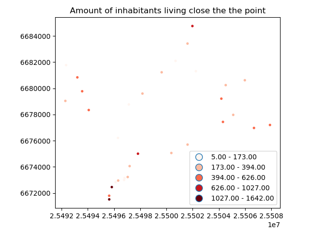
By knowing approximately how population is distributed in Helsinki, it seems that the results do make sense as the points with highest population are located in the south where the city center of Helsinki is.