Heatmaps with the Jupyter Gmaps plugin
Heatmaps are a good way of getting a sense of the density and clusters of geographical events. They are a powerful tool for making sense of larger datasets. The Jupyter **gmaps** plugin is a python library that work with the Google maps API to enable users to create great and meaningful maps.
The target in this part of the lesson is to:
- import csv file about offences against property (thefts, robbery etc) in Estonia
- create spatial geometry based on coordinates
- and then create a heatmap and visualise with
gmaps
Crime data is open data and originates from Estonian Police and Border Guard Board open data page. On the police website there are several different datasets for offenses and crimes, such as:
- Avaliku korra vastased ja avalikus kohas toime pandud varavastased süüteod: offenses committed against public order and in public places avalik_3.csv
- Varavastased süüteod: Offenses Against Property vara_1.csv
Environment Preparations
Activate your environments and install the jupyter Gmap plugin. The easiest way to install gmaps is with conda anyway:
(geopython-environment) C:\Users\Alexander\geopython> conda install -c conda-forge gmaps
Enable ipywidgets widgets extensions:
(geopython-environment) C:\Users\Alexander\geopython> jupyter nbextension enable --py --sys-prefix widgetsnbextension
Then tell Jupyter to load the extension with:
(geopython-environment) C:\Users\Alexander\geopython> jupyter nbextension enable --py --sys-prefix gmaps
Most operations on Google Maps require that you tell Google who you are. As the Gmaps plugin uses the Google Maps Java Script API a lot under the hood we need to follow the Authentication workflow and creating a key, and activate it
For todays lesson we will provide an API key that you’ll be able to use for the lesson. However, if you want to use it in other projects you should consider activating your own key, as we will disable this key soon again.
To authenticate with Google Maps, follow the Google API console instructions for creating an API key:
Data download and pre-processing
This Crime data we will use today is open data and regularly updated and published online at the same spot, so in order to add some more automation we will add the download of the data into our workflow.
# import common libraries
In [1]: import pandas as pd

In [2]: import geopandas as gpd

In [3]: from shapely.geometry import box, Polygon

In [4]: import numpy as np

# import the very practical urlib library from Python for web transactions, such as file download
In [5]: import urllib.request

# urlretrieve directly downloads the file into a local file handle
In [6]: local_file, headers = urllib.request.urlretrieve("https://opendata.smit.ee/ppa/csv/avalik_3.csv")
urlretrieve(url, filename) copies a network object denoted by a URL to a local file (API documentation here)
The function returns a tuple (filename, headers) where filename is the local file name under which the object can be found, because urlretrieve will save in some temporary folder.
And headers is a more technical information object containing status information for the http request and response.
You can also call urlretrieve(url, filename) with a second argument: if present, specifies the file location to copy to (if absent, the location will be a tempfile with a generated name, as seen above).
# read the CSV and strip whitespace
In [7]: df = pd.read_table(local_file)

# replace all empty strings with actual NoData values
In [8]: df[df == ""] = np.nan

# show the data
In [9]: df.head()
Out[9]:
                               JuhtumId    ...     SyyteoLiik
0  42964274-1636-18d5-8326-a9a756483dba    ...             KT
1  ec3a9088-1635-18d5-8326-a9a756483dba    ...             VT
2  ec3a6f36-1635-18d5-8326-a9a756483dba    ...             KT
3  429641ac-1636-18d5-8326-a9a756483dba    ...             VT
4  ec3a7e22-1635-18d5-8326-a9a756483dba    ...             KT

[5 rows x 18 columns]
We have many columns, for example:
- JuhtumId: just an Id for each event
- ToimKpv: date of the event
- ToimKell: time of the event
- ToimNadalapaev: weekday
- KohtLiik: a description of the locality where the event happened
- MaakondNimetus: Name of the county (maakond)
- ValdLinnNimetus: name of the municipality/city
- KohtNimetus: local place name/address
- Kahjusumma: monetary value of damage/offense
The data is provided in a normalised gridded fashion, the Lest_X and Y coordinate pairs give the lower and upper boundary of each corner of each grid-square polygon: - Lest_X: left and right (western, eastern) longitude boundary - Lest_Y: lower and upper (southern, northern) latitude boundary
You can see the coordinates are provided in a very awkward format, in x_min, x_max and y_min, y_max. But you can also recognise that they are in a projected CRS, because we don’t have GPS coordinates, but metric values that look like the Estonian national grid.
So we need a few steps in order to tease apart the values an build our polygons. Why, because in order to create a heatmap, we need a point dataset, and we will generate the points from the polygon centroids. For now we will use our well-known function syntax again:
In [10]: selected_cols = ['ToimKpv', 'ToimKell', 'ToimNadalapaev','KohtLiik','MaakondNimetus','ValdLinnNimetus','KohtNimetus','Kahjusumma','Lest_X','Lest_Y']

In [11]: df = df[selected_cols]

# just so that we can be sure that there are no NaN values for our coordinate work
In [12]: df.dropna(subset=['Lest_X', 'Lest_Y'], inplace=True)
We drop all the rows in which the columns ‘Lest_X’, ‘Lest_Y’ have these nan values, because we won’t be able to georeference them anyway.
- for each row, take the Lest_X and Lest_Y
- split the String into two fields using “-” as the point where to split
- construct a polygon from 4 points we can build from the separate coordinates
- return the polygon geometry and create the geometry column
In [13]: def construct_poly(row):
   ....:     lest_x = row['Lest_X']
   ....:     lest_y = row['Lest_Y']
   ....:     splitted_x_list = lest_x.split("-")
   ....:     splitted_y_list = lest_y.split("-")
   ....:     lower_y = int(splitted_y_list[0])
   ....:     upper_y = int(splitted_y_list[1]) + 1
   ....:     lower_x = int(splitted_x_list[0])
   ....:     upper_x = int(splitted_x_list[1]) + 1
   ....:     lower_left_corner = (lower_y, lower_x)
   ....:     lower_right_corner = (lower_y, upper_x)
   ....:     upper_right_corner = (upper_y, upper_x)
   ....:     upper_left_corner = (upper_y, lower_x)
   ....:     poly = Polygon([lower_left_corner, lower_right_corner, upper_right_corner, upper_left_corner, lower_left_corner])
   ....:     return poly
   ....:
We create this slightly more elaborate function in order to create the polygons out of the square-ish String coordinate pairs.
In [14]: df['geometry'] = df.apply(construct_poly, axis=1)

In [15]: df.head()
Out[15]:
      ToimKpv                        ...                                                                   geometry
0  2013-12-31                        ...                          POLYGON ((659000 6474000, 659000 6474500, 6595...
1  2013-12-31                        ...                          POLYGON ((473000 6534500, 473000 6535000, 4735...
2  2013-12-31                        ...                          POLYGON ((542500 6589000, 542500 6589500, 5430...
3  2013-12-31                        ...                          POLYGON ((686000 6589500, 686000 6590000, 6865...
4  2013-12-31                        ...                          POLYGON ((542000 6587500, 542000 6588000, 5425...

[5 rows x 11 columns]
We create a geodataframe from our dataframe using the Estonian national projected coordinate system.
In [16]: from fiona.crs import from_epsg

# we create a geodataframe from our dataframe using the Estonian national projected coordinate system
In [17]: gdf_3301_poly = gpd.GeoDataFrame(df, geometry='geometry', crs=from_epsg(3301))

# we'll also calculate the area
In [18]: gdf_3301_poly['area_m2'] = gdf_3301_poly.geometry.area

In [19]: gdf_3301_poly.head()
Out[19]:
      ToimKpv    ...      area_m2
0  2013-12-31    ...     250000.0
1  2013-12-31    ...     250000.0
2  2013-12-31    ...     250000.0
3  2013-12-31    ...     250000.0
4  2013-12-31    ...     250000.0

[5 rows x 12 columns]
In [20]: import matplotlib.pyplot as plt
In [21]: plt.style.use('ggplot')
In [22]: plt.rcParams['figure.figsize'] = (10, 7)
In [23]: plt.rcParams['font.family'] = 'sans-serif'
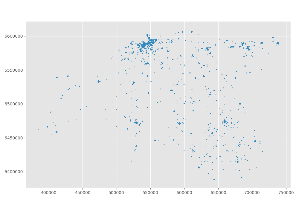
In [24]: gdf_3301_poly.plot()
Out[24]: <matplotlib.axes._subplots.AxesSubplot at 0x1501816df98>
In [25]: plt.tight_layout()

Then we convert L-EST to WGS84 (lon-lat), because the map plugin for gmaps will need lat lon coordinates (not projected). And because we will need points and not polygons for the heatmap, we calculate the centroid with a simple GeoDataframe function.
# convert L-EST to WGS84 (lon-lat), because the map plugon for gmaps will need lat lon coordinates (not projected)
In [26]: gdf_wgs84_poly = gdf_3301_poly.to_crs(epsg=4326)

# and because we will need points and not polygons for the heatmap, we calculate the centroid with a simple GeoDataframe function
In [27]: gdf_wgs84_poly['centroids'] = gdf_wgs84_poly.centroid

In [28]: gdf_wgs84_poly.head()
Out[28]:
      ToimKpv                     ...                                                         centroids
0  2013-12-31                     ...                       POINT (26.72285327135241 58.37963196028662)
1  2013-12-31                     ...                       POINT (23.53521336873965 58.95099743721788)
2  2013-12-31                     ...                       POINT (24.75340672472285 59.43891964444276)
3  2013-12-31                     ...                       POINT (27.28033777598366 59.40467512081494)
4  2013-12-31                     ...                       POINT (24.74430235856898 59.42550620159956)

[5 rows x 13 columns]
Some final steps before we can use the data for the gmaps heatmap function: We are required to provide a distinct list of lat/lon coordinate pairs and make sure there are no empty or NaN fields.
As we have centroids already prepared, we will clean the remaining dataframe and split the lat/lon fields off our centroids. Let’s prepare a simple function:
In [29]: def split_lat_lon(row):
   ....:     centerp = row['centroids']
   ....:     new_row = row
   ....:     new_row['lat'] = centerp.y
   ....:     new_row['lon'] = centerp.x
   ....:     return row
   ....:
And apply the function, and drop NaN fields along desired columns:
In [30]: gdf_wgs84_poly = gdf_wgs84_poly.apply(split_lat_lon, axis=1)

In [31]: gdf_wgs84_poly.head()
Out[31]:
      ToimKpv ToimKell    ...            lat        lon
0  2013-12-31    23:20    ...      58.379632  26.722853
1  2013-12-31    23:00    ...      58.950997  23.535213
2  2013-12-31    22:00    ...      59.438920  24.753407
3  2013-12-31    21:11    ...      59.404675  27.280338
4  2013-12-31    21:00    ...      59.425506  24.744302

[5 rows x 15 columns]
A quick statistical look at the data
Let’s define a few functions to sort out the month, the day of the week and the hour of the event time, as well as extracting the costs of damage into separate columns. This is always practical and helps us separating concerns we want to investigate in.
Python has a builtin datatime package which makes it easier for us to work with dates and times and converting between Strings (textual representation) and real chronological dat and time objects.
In [32]: from datetime import datetime

#
In [33]: noNanData = gdf_wgs84_poly.dropna(how = 'any', subset = ['ToimKell','ToimKpv','Kahjusumma','lon', 'lat','geometry']).copy()

#
In [34]: def getMonths(item):
   ....:     datetime_str = item
   ....:     datetime_object = datetime.strptime(datetime_str, '%Y-%m-%d')
   ....:     return datetime_object.month
   ....:

#
In [34]: def getWeekdays(item):
   ....:     datetime_str = item
   ....:     datetime_object = datetime.strptime(datetime_str, '%Y-%m-%d')
   ....:     return datetime_object.weekday()
   ....:

#
In [34]: def getHours(item):
   ....:     datetime_str = item
   ....:     datetime_object = datetime.strptime(datetime_str, '%H:%M')
   ....:     return datetime_object.hour
   ....:

#
In [34]: def getDamageCosts(item):
   ....:     try:
   ....:         lst_spl = item.split("-")
   ....:         lst_int = [int(i) for i in lst_spl]
   ....:         value = max(lst_int)
   ....:         return value
   ....:     except:
   ....:         return np.nan
   ....:
Then we apply the functions and create additional columns.
#
In [38]: noNanData['month'] = noNanData['ToimKpv'].map(lambda x: getMonths(x))
#
In [39]: noNanData['dayOfWeek'] = noNanData['ToimKpv'].map(lambda x: getWeekdays(x))
#
In [40]: noNanData['hour'] = noNanData['ToimKell'].map(lambda x: getHours(x))
#
In [41]: noNanData['costs'] = noNanData['Kahjusumma'].map(lambda x: getDamageCosts(x))
#
In [42]: print(noNanData.shape)
(23866, 19)
#
In [43]: noNanData.head()
������������Out[43]:
ToimKpv ToimKell ToimNadalapaev ... dayOfWeek hour costs
0 2013-12-31 23:20 Teisipäev ... 1 23 499.0
1 2013-12-31 23:00 Teisipäev ... 1 23 4999.0
2 2013-12-31 22:00 Teisipäev ... 1 22 499.0
4 2013-12-31 21:00 Teisipäev ... 1 21 499.0
5 2013-12-31 21:00 Teisipäev ... 1 21 499.0
[5 rows x 19 columns]
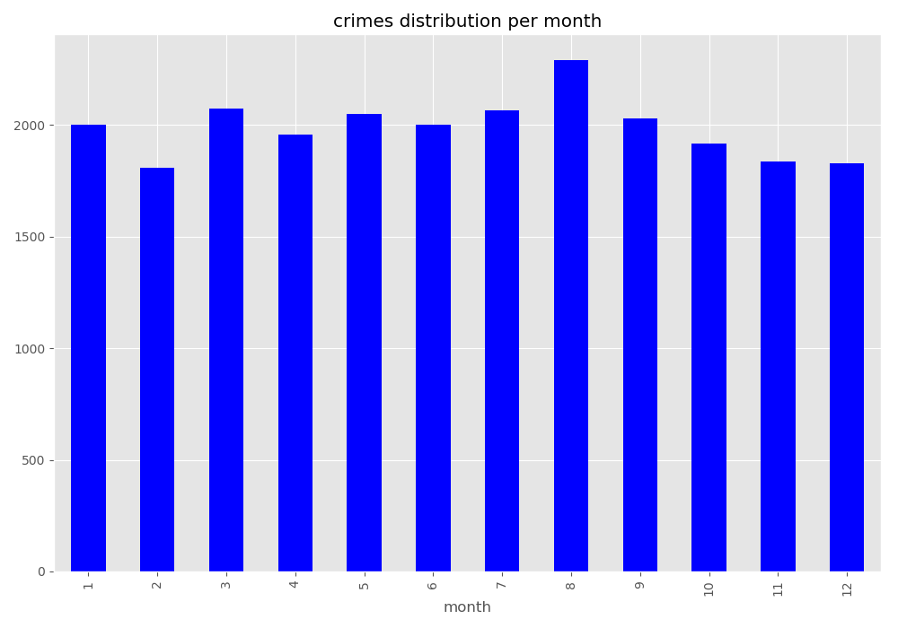
And then we can plot some different distributions of when the crimes happened…
In [44]: noNanData.groupby('month').size().plot(kind='bar', color='blue')
Out[44]: <matplotlib.axes._subplots.AxesSubplot at 0x1501e3eee10>
In [45]: plt.title("crimes distribution per month")
������������������������������������������������������������������Out[45]: Text(0.5, 1.0, 'crimes distribution per month')
In [46]: plt.tight_layout()

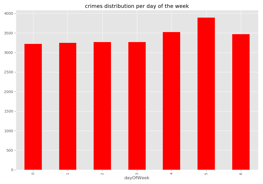
In [47]: print('Monday is 0 and Sunday is 6')
Monday is 0 and Sunday is 6
In [48]: noNanData.groupby('dayOfWeek').size().plot(kind='bar', color='red')
����������������������������Out[48]: <matplotlib.axes._subplots.AxesSubplot at 0x1501e3e5cf8>
In [49]: plt.title("crimes distribution per day of the week")
����������������������������������������������������������������������������������������������Out[49]: Text(0.5, 1.0, 'crimes distribution per day of the week')
In [50]: plt.tight_layout()

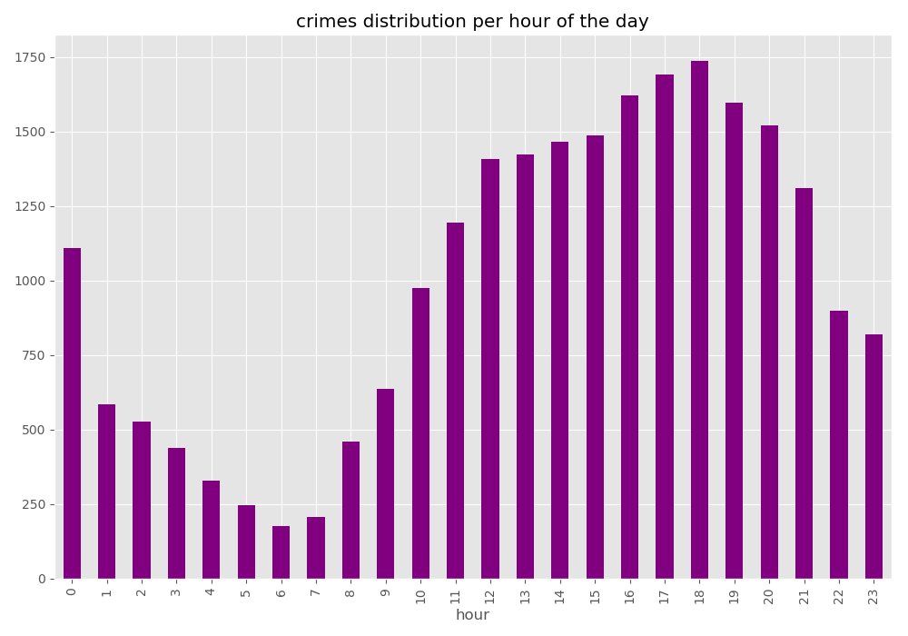
In [51]: noNanData.groupby('hour').size().plot(kind='bar', color='purple')
Out[51]: <matplotlib.axes._subplots.AxesSubplot at 0x1501e3be240>
In [52]: plt.title("crimes distribution per hour of the day")
������������������������������������������������������������������Out[52]: Text(0.5, 1.0, 'crimes distribution per hour of the day')
In [53]: plt.tight_layout()

… and what
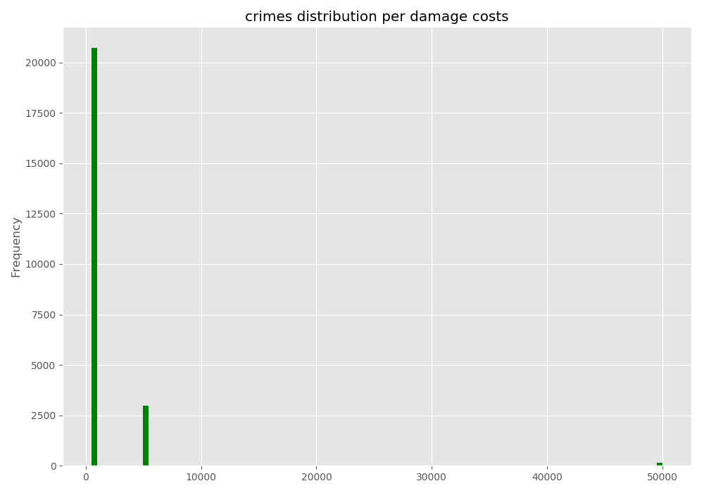
In [54]: noNanData["costs"].plot.hist(bins=100, color='green')
Out[54]: <matplotlib.axes._subplots.AxesSubplot at 0x1501e33c358>
In [55]: plt.title("crimes distribution per damage costs")
������������������������������������������������������������������Out[55]: Text(0.5, 1.0, 'crimes distribution per damage costs')
In [56]: plt.tight_layout()

Creating the Heatmap
Base configuration:
Most operations on Google Maps require that you tell Google who you are.
API key note
For the lesson we will provide an API key in Moodle!
To authenticate with Google Maps, follow the instructions for creating an API key. You will probably want to create a new project, then click on the Credentials section and create a Browser key. The API key is a string that starts with the letters AI.
import gmaps
# INPUTS
# Google API key of Alex
GOOGLE_API_KEY = 'xxx-code goes here'
#
gmaps.configure(api_key=GOOGLE_API_KEY)
Maps and layers created after the call to gmaps.configure will have access to the API key.
Note
A very good tutorial can be found on their website.
gmaps is built around the idea of adding layers to a base map. After you’ve authenticated with Google maps, you start by creating a figure,
which contains a base map and adding a list of coordinates as layer.
fig = gmaps.figure()

# gmaps.figure(map_type='HYBRID')
# gmaps.figure(map_type='TERRAIN')

# example_parameters
# 'city' is static and for close-up views, 'county' (default) is dissipating
#
# 'city': 'point_radius': 0.0075, 'max_intensity': 150, 'dissipating': False}
# 'county': {'point_radius': 29, 'max_intensity': 150, 'dissipating': True}

locations = noNanData[['lat', 'lon']]

heatmap_layer = gmaps.heatmap_layer(locations, point_radius=29, max_intensity=150, dissipating=True )
# heatmap_layer = gmaps.heatmap_layer(locations)

fig.add_layer(heatmap_layer)
fig
Preventing dissipation on zoom If you zoom in sufficiently, you will notice that individual points disappear. You can prevent this from happening by controlling the max_intensity setting. This caps off the maximum peak intensity. It is useful if your data is strongly peaked. This settings is None by default, which implies no capping. Typically, when setting the maximum intensity, you also want to set the point_radius setting to a fairly low value. The only good way to find reasonable values for these settings is to tweak them until you have a map that you are happy with.
heatmap_layer.max_intensity = 100
heatmap_layer.point_radius = 5
fig.add_layer(heatmap_layer)
fig
Setting the color gradient and opacity You can set the color gradient of the map by passing in a list of colors. Google maps will interpolate linearly between those colors. You can represent a color as a string denoting the color (the colors allowed by this):
heatmap_layer.gradient = [
    'white',
    'silver',
    'gray'
    ]

fig.add_layer(heatmap_layer)
fig
If you need more flexibility wit hsize and colour, you can try several of the more configuration options in the tutorial.
Weighted Heatmaps
By default, heatmaps assume that every row is of equal importance. You can override this by passing weights through the weights keyword argument. The weights array is an iterable (e.g. a Python list or a Numpy array) or a single pandas series. Weights must all be positive (this is a limitation in Google maps itself).
https://jupyter-gmaps.readthedocs.io/en/latest/tutorial.html#weighted-heatmaps
fig = gmaps.figure()
heatmap_layer = gmaps.heatmap_layer(
    noNanData[['lat', 'lon']], weights=noNanData['costs'],
    max_intensity=30, point_radius=3.0
)
fig.add_layer(heatmap_layer)
fig