library(sf)       # for working with spatial data
library(tidyverse)# for data manipulation and visualization
library(tmap)     # for creating static and interactive maps
library(osmdata)  # to access OpenStreetMap data
library(units) # for handling measurement unitsLesson 2: Vector data analysis (Part 1)
This lesson covers the fundamental aspects of working with vector data in R. It encompasses understanding of sf objects and their structures, managing CRSs for vector data, and conducting spatial queries on diverse geometric features using the sf package’s functions.
Learning outcomes
At the end of this lesson, the students should be able to:
- Understand and work with various sf data types
- Manage CRS for vector data effectively
- Perform spatial queries on a variety of geometric features
Let’s start the lesson by installing and loading the required packages. Starting each R session by loading the required packages is a good practice to ensure efficient and well-organized workflows. We’ll begin this and upcoming lessons by loading the necessary packages. It’s essential to know that we may not initially be aware of all the packages needed, thus the list of the packages may evolve as we progress through the lesson.
Please note that thesf and tidyverse packages were installed in lesson 1, allowing you to load them directly. However, for any new packages, such as tmap, osmdata, and units, that haven’t been installed yet, you’ll need to install them before loading
2.1. Simple Features and their structures
Simple Features or simple feature access is a standardized way to represent and manipulate spatial vector data in R. It provides a standardized way to work with geographic or geometric objects, such as points, lines, and polygons, along with associated attributes. In other words, simple features (sf) is a formal standard set of guidelines established by both the Open Geospatial Consortium (OGC) and International Organization for Standardization(ISO) that describes how objects in the real world can be represented in computers. It provides a consistent framework for working with geometric objects, making it easier to perform operations like spatial data analysis, visualization, and integration with other data.
In R, the sf package is the primary tool for handling sf data. The sf package provides extensive capabilities for working with vector data, including reading, writing, and manipulation. All functions and methods in sf that operate on spatial data are prefixed by st_, which refers to spatial type. Simple features generally comprise a total of 18 geometry types, but the following seven and their combination are the most prevalent and frequently employed in the majority of GIS analyses.

There are three classes commonly used to represent simple features in geospatial data:
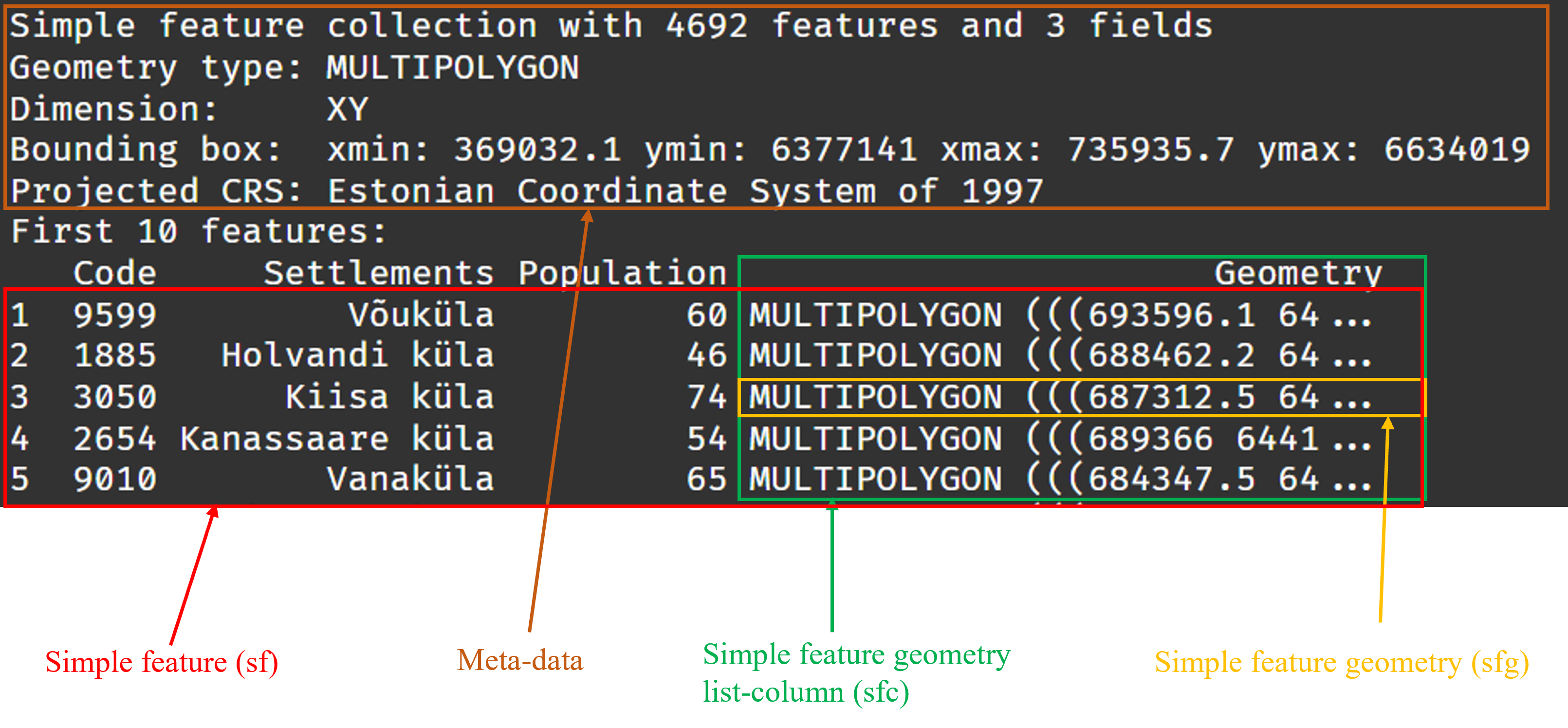
sfg (Simple Features Geometry): represents the geometry of a single feature, such as a point, linestring, or polygon. It is used to store a single geometric shape (e.g., a single point or a single line) along with its attributes.sfc (Simple Feature Geometry List-Column): represents collections of one or more geometric objects (sfg) of the same type. It is used to group multiple geometries of the same type into a single object. For example, you can use sfc to represent a collection of multiple points, a collection of multiple lines, or a collection of multiple polygons.sf (Simple Features): represents complete spatial datasets, combiningattributedata withgeometriesin a data frame. An sf object can hold multiple features (e.g., multiple points, lines, or polygons) and associated attributes in a tabular format.
The figure below depicts the general structure of sf object classes:

As depicted in the diagram, the initial step involves the creation of each feature’s geometry using specific constructor functions. These features will belong to the sfg class, representing simple feature geometries. Subsequently, we assemble all these geometries into a list using the st_sfc() function, resulting in a new object classified as sfc or a simple feature list-column. Finally, we merge this newly created sfc with the attributes (stored as a data frame, or a tibble) using the st_sf() function to get an sf object.
To gain a better understanding of the arrangement of different feature classes, refer the diagram below, which illustrates the first few observations from the pop_new_filled_sf object introduced in lesson 1.
2.2. Creating spatial objects
Let’s create simple feature classes from scratch using user-defined coordinates and the sf package. This approach will enhance our understanding of the various types of simple feature geospatial data and the methods for transitioning between different class types.
First, we will create point geometry using st_multipoint() function and then generate LINESTRING and POLYGON geometries from point geometry using st_cast() function. The st_cast() is a function used for casting or converting geometries from one type to another while preserving the essential spatial relationships.
# Create the longitude and latitude vectors
lon <- c(24.0, 24.2, 24.4, 24.5, 24.7, 24.6, 24.4, 24.3, 24.0)
lat <- c(57.0, 57.2, 57.1, 57.3, 57.5, 57.6, 57.8, 57.7, 57.6)

# Combine the longitude and latitude vectors into a matrix
coordinates <- cbind(lon, lat)

# Create point geometry
points <- st_multipoint(coordinates)
linestring <-  st_cast(points, "LINESTRING")
polygon <-  st_cast(points, "POLYGON")
polygon
POLYGON ((24 57, 24.2 57.2, 24.4 57.1, 24.5 57.3, 24.7 57.5, 24.6 57.6, 24.4 57.8, 24.3 57.7, 24 57.6, 24 57))# Check the classes
class(points)[1] "XY" "MULTIPOINT" "sfg" We have successfully created sfg objects containing multiple points, linestrings and polygon. These geometries are represented in two dimensions (2D) as “XY” coordinates. However, it’s worth noting that spatial data can also include additional dimensions such as “Z” for altitude and “M” for some measure. In situations where the object includes a third dimension (Z or M), R might encounter issues during processing. To address this, you can use the st_zm() function to handle and manipulate the third dimension appropriately.
Now we need to collect the geometries inside sfg objects and create sfc objects using st_sfc() function.
# Collect geometries inside sfg objects
point_sfc <- st_sfc(points)
lines_sfc <- st_sfc(linestring)
poly_sfc <- st_sfc(polygon)
poly_sfc
Geometry set for 1 feature
Geometry type: POLYGON
Dimension: XY
Bounding box: xmin: 24 ymin: 57 xmax: 24.7 ymax: 57.8
CRS: NAPOLYGON ((24 57, 24.2 57.2, 24.4 57.1, 24.5 57....# Check the classes
class(point_sfc)[1] "sfc_MULTIPOINT" "sfc" The sfg objects have now been transformed into sfc objects that include coordinate reference system (CRS) information. Our sfc objects are actually a list (check using typeof()) which can be used to extract individual elements if needed. However, sfc objects do not carry additional attributes or data, they are more lightweight compared to sf objects. To make our spatial data analysis more effective, we need to convert the sfc object to the more commonly used sf class.
As a last step, let’s combine the feature geometries with the related attributes using the st_sf() function and create GIS data set stored as an sf object.
# Collect geometries inside the sfc objects
points_sf <- st_sf(point_sfc)
lines_sf <- st_sf(lines_sfc)
polygon_sf <- st_sf(poly_sfc)
polygon_sf
Simple feature collection with 1 feature and 0 fields
Geometry type: POLYGON
Dimension: XY
Bounding box: xmin: 24 ymin: 57 xmax: 24.7 ymax: 57.8
CRS: NA
poly_sfc
1 POLYGON ((24 57, 24.2 57.2,...# Check the class
class(points_sf)[1] "sf" "data.frame"# We can also check the type of geometry
st_geometry_type(polygon_sf) [1] POLYGON
18 Levels: GEOMETRY POINT LINESTRING POLYGON MULTIPOINT ... TRIANGLEGreat! We’ve successfully created ‘sf’ objects from scratch and explored geometry class conversions. Now, let’s visualize these objects together using the standard R ‘plot()’ function.”
# Plot the point, line and polygon geometries together
plot(polygon_sf,  col="#CD853F", axes = TRUE)
plot(lines_sf, add = TRUE, col = "#0000CD", lwd=3)
plot(points_sf, add = TRUE,  col = "#DC143C", pch=20, cex=2)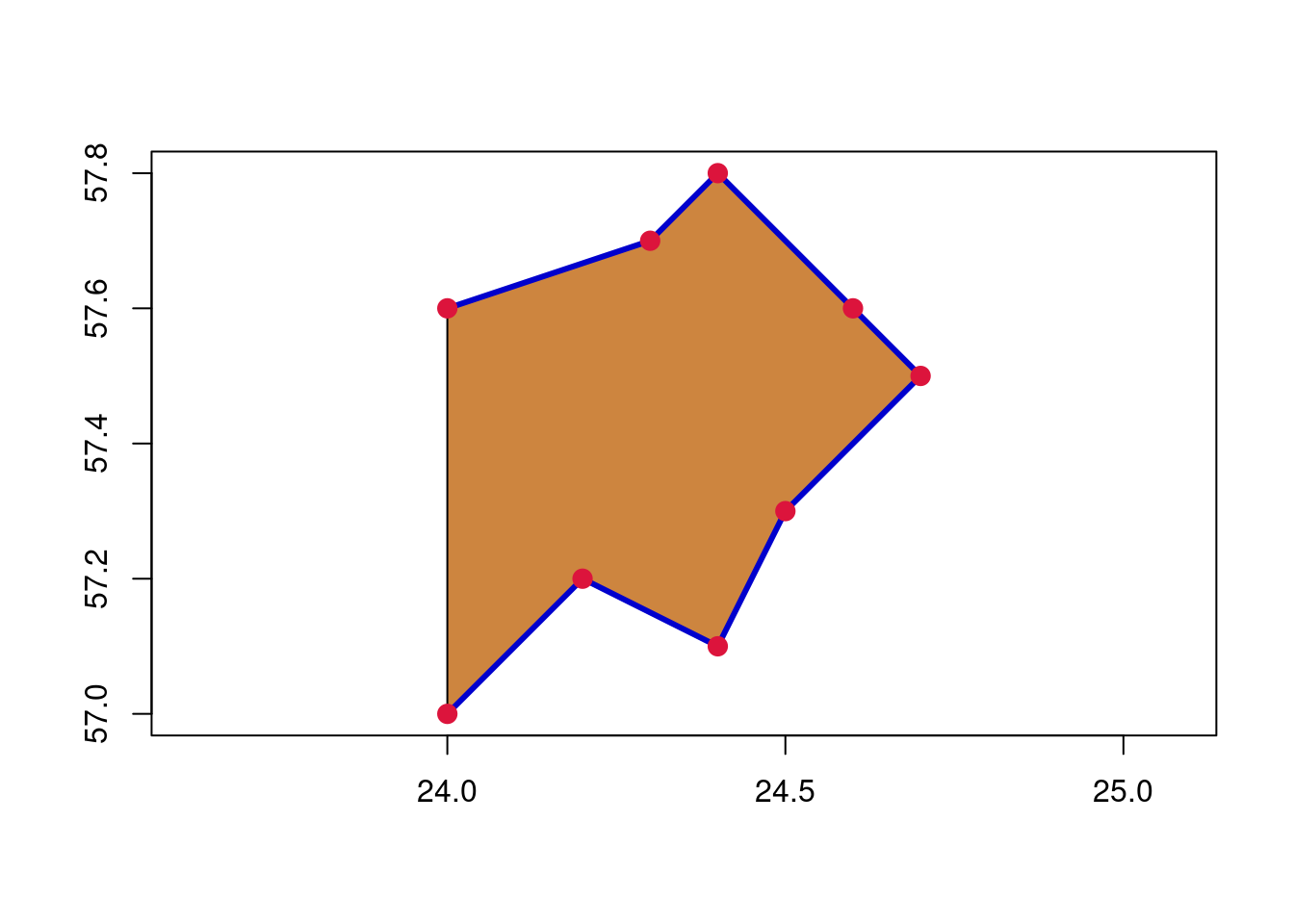
Before starting any spatial analysis operations with sf objects, it is important to check their geometric validity. While official datasets are generally expected to be valid, this is not always the case. Working with invalid geometries can introduce challenges in certain analyses, such as computing areas. Points and Lines are always valid. However, polygons may exhibit invalidity, primarily when they contain self-intersections. Please check this link for a few examples of invalid geometries.
The st_is_valid() function from sf package enables us to check the geometric validity of the objects. Let’s check the geometric validity of our polygon_sf object:
# Check if the polygon is valid
st_is_valid(polygon_sf)
[1] TRUE# add the argument `reason = TRUE` to get a short description
st_is_valid(polygon_sf, reason = TRUE)[1] "Valid Geometry"In case, your geometry is invalid, the st_make_valid() function can be used to make it valid according to the simple features standard.
2.3. Coordinate Reference Systems (CRSs) in R
A very important aspect of spatial data is using coordinate reference systems. CRSs can be broadly categorized into two types: geographic and projected. However, we won’t get into the details here, as you have already extensively covered this topic in lesson 2 of the Python classes. For further insights, you may also refer to this link.
CRSs have unique ID-s - EPSG codes the EPSG numeric code which help to identify specific CRS and it’s parameters. To look up EPSG code of your interest, just go to this link and search for it. For example, EPSG code for Estonia can be found here - epsg projection 3301 - estonian coordinate system of 1997. The official CRS of Estonia is L-EST97, EPSG:3301.
2.3.1. Identifying and assigning CRSs
When working with geospatial data, you should always firstly check (identify) it’s CRS.
Let’s inspect the CRS of our previously created polygon_sf object using the st_crs() function from the sf package.
st_crs(polygon_sf) Coordinate Reference System: NAThe output indicates that the CRS has not been defined or assigned to the spatial object. As we created the data ourselves but did not specify what CRS it is then we can assign CRS. Since we used geographic coordinates to create polygon_sf object, we can assign the data WGS84 CRS. If we would have obtained the data from someone else and it does not have CRS information, then you must be absolutely sure in what CRS it is before assigning the CRS. Otherwise you will ruin the data.
Let’s assign the polygon_sf object to World Geodetic System (WGS84; EPSG:4326). We can use two different functions: st_set_crs() or st_crs()
# Assign the CRS using st_crs() directly
st_crs(polygon_sf) <- 4326

# Create a new object with the CRS using st_set_crs()
polygon_sf_4326 <- st_set_crs(polygon_sf, 4326)

# Assign the CRS of points_sf to match the CRS of polygon_sf_4326
st_crs(points_sf) <- st_crs(polygon_sf_4326)
polygon_sf_4326
Simple feature collection with 1 feature and 0 fields
Geometry type: POLYGON
Dimension: XY
Bounding box: xmin: 24 ymin: 57 xmax: 24.7 ymax: 57.8
Geodetic CRS: WGS 84
poly_sfc
1 POLYGON ((24 57, 24.2 57.2,...The output confirms that WGS84 has been assigned to our polygon_sf_4326 as coordinate reference system (i.e. coordinates are in decimal degrees (lat, lon)). To check if polygon_sf_4326 uses geographic (longitude/latitude) or planar (projected) coordinates, we can use st_is_longlat().
st_is_longlat(polygon_sf_4326)[1] TRUE2.3.2. Reprojecting vector data
In most cases, you will work with the data that has CRS already assigned. However, if we are working with multiple data sources and different regions, we need to reproject the data from one CRS to another. A lot of data is nowadays obtained through satellites or GPS and this data is in WGS84 (geographic CRS). However, to perform spatial analysis or make maps, you need to project the data into your national or regional projected CRS.
In R, reprojecting vector data is straightforward using the st_transform() function from the sf package.
As we are working with Estonian data then let’s reproject polygon_sf_4326from WGS84 (EPSG:4326) to Estonian National CRS L-EST97 (EPSG:3301):
# Transform the polygon_sf_4326 object to L-EST97
polygon_sf_3301 <- st_transform(polygon_sf_4326, 3301)
polygon_sf_3301
Simple feature collection with 1 feature and 0 fields
Geometry type: POLYGON
Dimension: XY
Bounding box: xmin: 5e+05 ymin: 6317349 xmax: 541973.4 ymax: 6406530
Projected CRS: Estonian Coordinate System of 1997
poly_sfc
1 POLYGON ((5e+05 6317349, 51...Now we have reprojected our object from its original geographic (EPSG:4326) to a projected (EPSG:3301) coordinate system, resulting in coordinate units as meters. The st_is_longlat(polygon_sf_3301) now will return FALSE.
st_is_longlat(polygon_sf_3301)[1] FALSEWith the reprojected object, we can now perform some spatial operations, for example calculating the area and centroid of the polygon. In R, area of polygons can be computed using the st_area() function in sf package. It returns the area of the polygon, which is commonly measured in square meters.
# Calculate the area of polygon_sf_3301
area_polygon <- st_area(polygon_sf_3301)
area_polygon
2108027772 [m^2]We can change the unit of area from meters to a larger unit, such as square kilometers, by employing the set_units() function from the units package.
# Convert the area to sq. km
area_polygon <- units::set_units(area_polygon, km^2)
area_polygon
2108.028 [km^2]Computing the centroid of polygons is another common operation which involves finding the geometric center of a polygon, which can be useful in various spatial analysis and mapping tasks. In R, centroids can be easily computed using the st_centroid() function.
# Calculate the centroid of the 'polygon_sf_3301' object
polygon_centroid <- st_centroid(polygon_sf_3301)
Let’s plot the polygon_centroid object together with the polygon_sf_3301 object (polygon geometry):
# Plot the polygon_sf_3301 object in a specific color with axes
plot(polygon_sf_3301, col = "#CD853F", axes = TRUE)

# Add the centroid to the existing plot in red, with a specific point character (pch) and size (cex)
plot(polygon_centroid, add = TRUE, col = "#8B0000", pch = 20, cex = 2)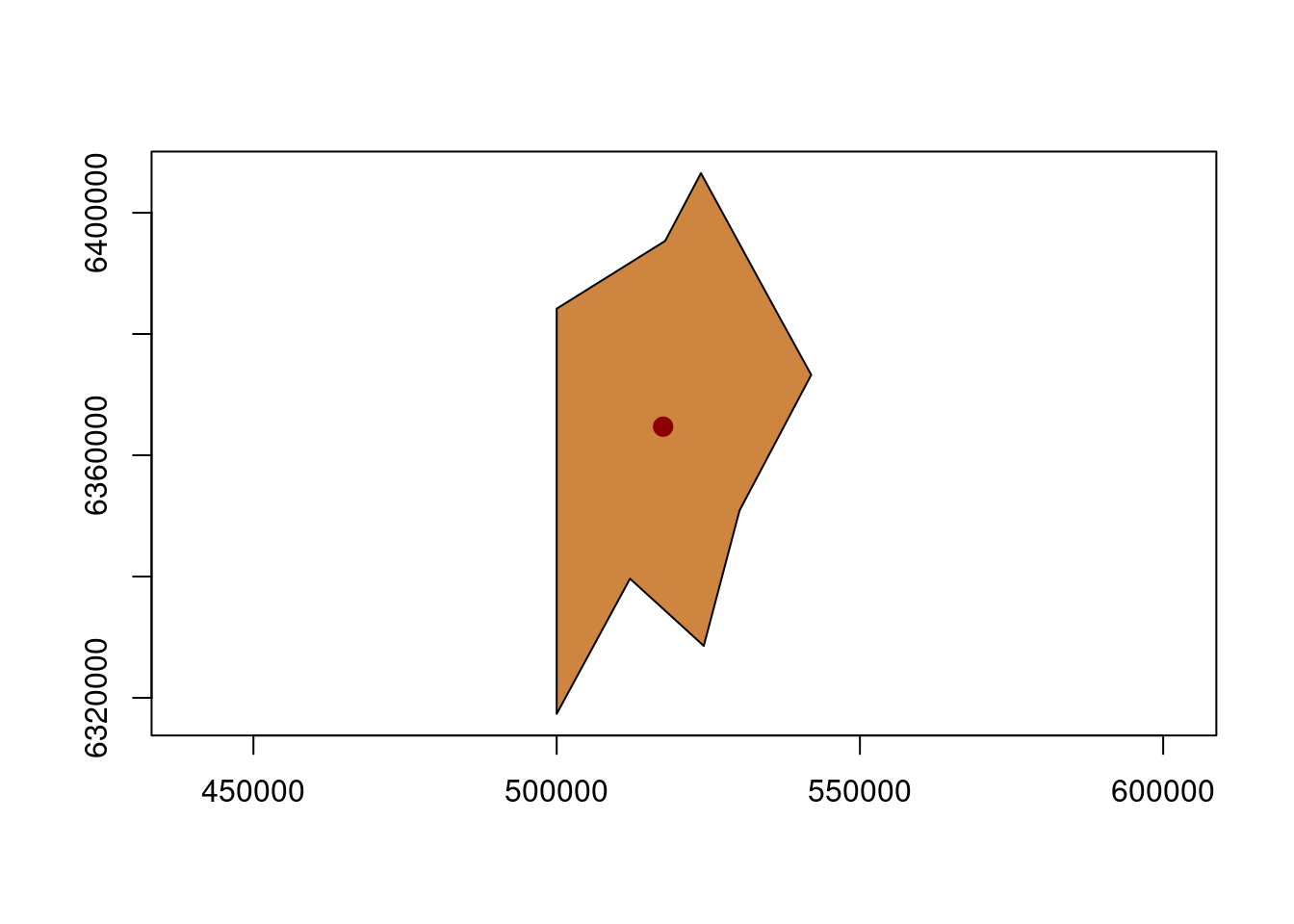
2.4. Spatial queries in R
Spatial query refers to a statement or logical expression that selects geographic features based on location or spatial relationship. In other words, it is the process of retrieving, analyzing, or manipulating geographic data (such as points, lines, polygons) based on their spatial characteristics.
In this lesson, we will explore several commonly used spatial queries using datasets that include information about Tartu bike stations and districts, obtained from the Tartu city government, as well as data related to Tartu shops and the Emajõgi river downloaded from OpenStreetMap using the osmdata package.
Let’s start with downloading the OSM datasets. The osmdata package in R provides a straightforward method to retrieve OSM data.
The available_features() function from osmdata package enables use to get the list of features in OSM.
available_features()The available_tags() function provides additional information about specific geographic features:
available_tags("shop") # the available_tags() function is used to retrieve a list of the available OSM tags (i.e., metadata) for specific geographic elements (e.g, shop). # A tibble: 174 × 2
Key Value
<chr> <chr>
1 shop [[ Too many Data Items entities accessed. | motorcycle ]]
2 shop agrarian
3 shop alcohol
4 shop anime
5 shop antiques
6 shop appliance
7 shop art
8 shop atv
9 shop baby_goods
10 shop bag
# ℹ 164 more rowsThe first step in the process of obtaining data using the osmdata package is to define area of interest, which can be done by specifying either a bounding box or the name of the place. The osmdata package has a convenient function known as getbb() that is specifically designed to retrieve the bounding box of a location based on its name.
# Defining the bounding box for Tartu city
tartu_bb <- osmdata::getbb("Tartu")
After the area is defined, the next step is creating an overpass query as osmdata package retrieves data by using the Overpass API, which provides custom-selected segments of the OSM map data in a read-only manner. This can be easily done using the opq() function of the osmdata package.
Let’s use bounding box object (tartu_bb) to create the overpass query:
# Creating an overpass query
tartu_opq <- tartu_bb %>%
  opq()
After configuring the Overpass API, the next step is incorporating essential features and tags into the query, which can be achieved by using the add_osm_feature() function. To obtain the data in a more accessible format for subsequent analysis, the osmdata_sf() function allows us to retrieve it in the form of simple features.
# Retrieving shops and storing it as an sf object
tartu_shops <- tartu_opq %>%
  add_osm_feature(key = "shop") %>%
  osmdata_sf()  # store as simple features data f

# Retrieving rivers and storing it as an sf object
tartu_rivers <- tartu_opq %>%
  add_osm_feature(key = "waterway", value = "river") %>%
  osmdata_sf()

# Check the class
class(tartu_shops)
[1] "list" "osmdata" "osmdata_sf"# Convert osmdata_sf to sf
shops_sf <- st_as_sf(tartu_shops$osm_points)
rivers_sf <- st_as_sf(tartu_rivers$osm_lines)
# Inspect the summary of the datasets
#glimpse(shops_sf)
#glimpse(rivers_sf)The dataset rivers_sf contains multiple disjoint river lines. In this tutorial, our target is to retrieve the Emajõgi river, which intersects the Tartu district. The following code extracts only Emajõgi river and merges its segments into a unified, continuous line.
# Select the river segments for "Emajõgi"
emajogi <- rivers_sf %>%
  filter(name == "Emajõgi")

# Dissolve the segments into a single line based on the "name" attribute
emajogi_single_line <- emajogi %>%
  st_union()

# Convert sfc objects to sf objects and specify the attribute data
ema_riv <- st_sf(emajogi_single_line)
If you inspect the shops_sf dataset using glimpse function, you can observe that it comprises a total of 102 variables (please note that the number of variables may vary each time you execute an overpass query). However, our primary aim is to extract the location information for the shops, denoted by the geometry column. To clean up our data, we will retain only the osm_id and geometry columns while dropping others.
# Select osm_id and name columns from shops_sf object
shops_new <- shops_sf %>%
  dplyr::select(osm_id, geometry)

# Display the structure
glimpse(shops_new)
Rows: 1,390
Columns: 2
$ osm_id <chr> "266921299", "322906403", "326236651", "330809479", "33102367…
$ geometry <POINT [°]> POINT (26.67666 58.35805), POINT (26.73024 58.38247), P…Let’s visualize the river and shops datasets together using tmap and examine them more closely. tmap is a package designed for creating thematic maps in R. Throughout this course, we will make use of this package to generate both static and interactive maps. For additional information, please refer to the documentation here. Choosing between static plotting and interactive viewing in tmap can be achieved by configuring the tmap_mode() function with the respective options: tmap_mode("plot") for static plotting and tmap_mode("view") for interactive viewing.
# Create visualization
tmap_mode("view")  # set interactive plotting
tmap mode set to interactive viewingtm_shape(shops_new) +
tm_symbols(col = "#8B0000") +
tm_shape(ema_riv) +
tm_lines(col = "#0000FF",
lwd = 2) +
tm_layout(frame = FALSE) We can now move forward by importing the remaining datasets, which include the districts and bike stations. Please download the districts data from this link and the bike stations data from this link, and save the files in the same directory as the R script file (R_02 folder).
# Import districts
districts <- st_read("tartu_districts.gpkg")
Reading layer `tartu_districts' from data source
`/home/geoadmin/dev/simply-general/teaching/geospatial_python_and_r/R_02/tartu_districts.gpkg'
using driver `GPKG'
Simple feature collection with 33 features and 2 fields
Geometry type: MULTIPOLYGON
Dimension: XY
Bounding box: xmin: 655873.6 ymin: 6469758 xmax: 663717.9 ymax: 6477657
Projected CRS: Estonian Coordinate System of 1997# Display the structure
glimpse(districts)Rows: 33
Columns: 3
$ OBJECTID <dbl> 14, 34, 23, 12, 1, 41, 22, 38, 39, 7, 30, 37, 9, 8, 31, 36, 2…
$ NIMI <chr> "Veeriku tööstuse", "Sadama", "Jalaka", "Tähtvere", "Ees-Anne…
$ geom <MULTIPOLYGON [m]> MULTIPOLYGON (((656264.1 64..., MULTIPOLYGON (((…# Import bike stations
stations <- st_read("bike_stations.gpkg")Reading layer `tartu_bike_share_stations' from data source
`/home/geoadmin/dev/simply-general/teaching/geospatial_python_and_r/R_02/bike_stations.gpkg'
using driver `GPKG'
Simple feature collection with 101 features and 8 fields
Geometry type: POINT
Dimension: XY
Bounding box: xmin: 649813.2 ymin: 6467043 xmax: 668519.4 ymax: 6478854
Projected CRS: Estonian Coordinate System of 1997# Display the structure
glimpse(stations)Rows: 101
Columns: 9
$ OBJECTID <dbl> 6468, 6470, 6473, 6810, 6811, 6812, 6813, 6815, 6816, 6817…
$ Rataste_arv <int> 20, 20, 20, 16, 18, 15, 12, 8, 16, 12, 9, 15, 8, 12, 9, 20…
$ Asukoht <chr> "79 E-kaubamaja", "76 Tartu Maja", "72 Paju", "10 Turusild…
$ Markus <chr> NA, NA, NA, NA, NA, NA, NA, NA, NA, NA, NA, NA, NA, NA, NA…
$ Omanik <int> 3, 3, 3, 3, 3, 3, 3, 3, 3, 3, 3, 3, 3, 3, 3, 3, 3, 3, 3, 3…
$ Staatus <int> 1, 1, 1, 1, 1, 1, 1, 1, 1, 1, 1, 1, 1, 1, 1, 1, 1, 1, 1, 1…
$ P_aasta <int> 2020, 2020, 2020, 2019, 2019, 2019, 2019, 2019, 2019, 2019…
$ Linnaosa <int> 4, 16, 17, 1, 1, 1, 1, 1, 1, 1, 3, 17, 7, 7, 7, 5, 5, 13, …
$ geom <POINT [m]> POINT (659812.7 6472137), POINT (657050.9 6474397), …Now, we can create an interactive map that displays all the datasets we’ve gathered for this lesson.
# visualize districts, stations, shops, and rivers using tmap
tmap_mode("view") # set interactive plotting
tmap mode set to interactive viewingall_in1 <- tm_shape(districts) +
tm_polygons(col = "#CDC0B0") +
tm_shape(stations) +
tm_symbols(col = "#8B0000",
size = 0.1,
shape = 16) +
tm_shape(shops_new) +
tm_symbols(col = "#000000",
size = 0.1,
shape = 16)+
tm_shape(ema_riv)+
tm_lines(col = "#0000FF",
lwd = 2)
all_in1With all the essential datasets now prepared and organized to meet our analysis needs, we can transition seamlessly into executing spatial queries.
2.4.1. Point-in-polygon
A point-in-polygon query involves the determination of whether a point falls within a defined geographical area (polygon). Typically, this spatial query serves as one of the initial steps in a spatial analysis workflow.
The sf package in R offers two distinct methods for performing point-in-polygon queries:
st_within(): checks if one geometry is completely inside another geometry. In a Point-in-Polygon query, st_within() will return true if the point is inside the polygon and false if it’s outside or on the boundary of the polygon.st_contains(): checks if one geometry contains another. In a Point-in-Polygon query, it returns true if the polygon completely contains the point.
Your choice between these functions may depend on the specific requirements of your use case. If you have numerous points and a single polygon, and you aim to identify which points fall inside the polygon, st_within() is the suitable choice. On the other hand, if you have multiple polygons and a single point, and you want to determine which polygon contains the point, then st_contains() is the appropriate function to employ.
Let’s create a point-in-polygon query to determine if any of the bike stations are situated within the Kesk-Annelinna district, using the districts object.
# Filter the Kesk-Annelinna district
ka_dist <- districts %>%
  filter(NIMI =="Kesk-Annelinna")

ka_dist
Simple feature collection with 1 feature and 2 fields
Geometry type: MULTIPOLYGON
Dimension: XY
Bounding box: xmin: 660427.5 ymin: 6472904 xmax: 662852.8 ymax: 6474470
Projected CRS: Estonian Coordinate System of 1997
OBJECTID NIMI geom
1 37 Kesk-Annelinna MULTIPOLYGON (((661984.2 64...Next, apply the st_within() function to select all stations that fall within our specified polygon (Kesk-Annelinna) boundary:
# Check if there are any stations within the Kesk-Annelinna district
stations_ka_dist <- st_within(stations, ka_dist, sparse = FALSE)

# try by reversing the input order ("st_within(ka_dist, stations, sparse = FALSE)")

# sparse = FALSE specifies whether the result should be a sparse logical matrix (sparse = TRUE) or a regular logical matrix (sparse = FALSE).

# Inspect the structure
glimpse(stations_ka_dist)
logi [1:101, 1] FALSE FALSE FALSE FALSE TRUE TRUE ...The result of the code above provides a matrix consisting of 101 rows and 1 column. Each row represents a station, and the column corresponds to the Kesk-Annelinna district. If the value in a cell is TRUE, it indicates that the respective station falls within the target district’s boundary, and FALSE value signifies the opposite. We have a single vector, as we are identifying stations within a single district polygon.
Now, let’s extract only the stations that fall within the Kesk-Annelinna district (i.e., rows where the cell value is TRUE).
# Filter station that fall within the Kesk-Annelinna district
stations_within_ka <- stations[stations_ka_dist, ]
glimpse(stations_within_ka)
Rows: 11
Columns: 9
$ OBJECTID <dbl> 6811, 6812, 6813, 6815, 6816, 6817, 6876, 6877, 14084, 140…
$ Rataste_arv <int> 18, 15, 12, 8, 16, 12, 12, 12, 20, 14, 14
$ Asukoht <chr> "1 Kalda tee", "2 Kaunase puiestee", "3 Annelinna keskus",…
$ Markus <chr> NA, NA, NA, NA, NA, NA, NA, NA, NA, NA, NA
$ Omanik <int> 3, 3, 3, 3, 3, 3, 3, 3, 3, 3, 3
$ Staatus <int> 1, 1, 1, 1, 1, 1, 1, 1, 1, 1, 1
$ P_aasta <int> 2019, 2019, 2019, 2019, 2019, 2019, 2019, 2019, 2022, 2019…
$ Linnaosa <int> 1, 1, 1, 1, 1, 1, 1, 1, 1, 1, 1
$ geom <POINT [m]> POINT (661007.8 6473687), POINT (661676.9 6473471), POINT …Now we have identified nine stations that fall within the boundary of the Kesk-Annelinna district. Let’s visualize these stations along with the districts data.
# Plot the intersecting districts
tmap_mode("plot")
tmap mode set to plottingka_map <- tm_shape(districts) +
tm_polygons(col = "#CDC0B0")+
tm_shape(stations_within_ka) +
tm_symbols(col = "#8B0000", size = 0.5) +
tm_layout(frame = FALSE)
ka_map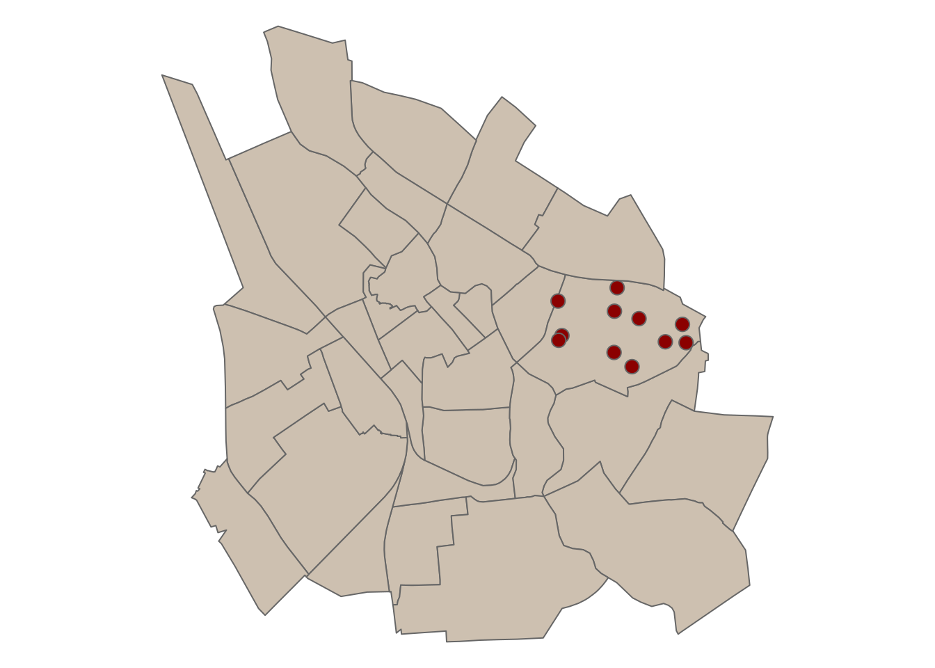
Exercise (10 minutes)
In our previous query, we have explored how to verify if any stations are locatedwithinthe Kesk-Annelinna district. Now, let’s switch our perspective and focus on checking if the Kesk-Annelinna districtcontainsany stations.
- Find stations contained by Kesk-Annelinna and visualize the result using tmap (Hint: use
st_contains()function).- Does the result of this query differ from our previous query using the
st_within()function? If not, what is the difference between the two queries?
2.4.2. Intersection
Another commonly used spatial query in GIS is determining the intersection between geometries, e.g., a line and polygon. Such query helps identify the parts of a line (such as roads, rivers, or boundaries) that intersect with a specific polygon or set of polygons (like administrative boundaries, land parcels, or geographic regions).
Let’s find districts that intersect with the Emajõgi river using st_intersects function:
# Transform 'ema_river' to match the CRS of 'districts' (CRS 3301)
ema_riv_3301 <- st_transform(ema_riv, crs = 3301)

# Calculate spatial intersections between districts and the transformed river
dis_riv_intersect <- st_intersects(districts, ema_riv_3301, sparse = FALSE)

# Display the summary
glimpse(dis_riv_intersect)
logi [1:33, 1] FALSE TRUE FALSE TRUE TRUE FALSE ...The above code returns a logical vector in which each element corresponds to a district in the districts dataset. When a district intersects with the river, it is assigned a TRUE value; conversely, if there is no intersection, it is assigned a FALSE value.
Let’s filter out the districts that intersect the river only:
# Filter the names of districts intersecting Emajõgi
intersect_dist_names <- districts[dis_riv_intersect,]
intersect_dist_names
Simple feature collection with 15 features and 2 fields
Geometry type: MULTIPOLYGON
Dimension: XY
Bounding box: xmin: 656730.6 ymin: 6469758 xmax: 663418.3 ymax: 6477657
Projected CRS: Estonian Coordinate System of 1997
First 10 features:
OBJECTID NIMI geom
2 34 Sadama MULTIPOLYGON (((660026 6473...
4 12 Tähtvere MULTIPOLYGON (((658612.5 64...
5 1 Ees-Annelinna MULTIPOLYGON (((660427.5 64...
8 38 Taga-Annelinna MULTIPOLYGON (((662827.4 64...
11 30 Vanalinna MULTIPOLYGON (((659403.4 64...
12 37 Kesk-Annelinna MULTIPOLYGON (((661984.2 64...
13 9 Ülejõe MULTIPOLYGON (((660440.1 64...
16 36 Ujula MULTIPOLYGON (((658368.5 64...
19 11 Supilinn MULTIPOLYGON (((659169.3 64...
20 15 Uueturu MULTIPOLYGON (((659696.2 64...Let’s generate a visualization that displays the districts intersecting with the Emajõgi river alongside the complete set of districts.
# Plot the intersecting districts
tmap_mode("plot")
tmap mode set to plottingtm_shape(districts) +
tm_polygons(col = "#CDC0B0")+
tm_shape(intersect_dist_names) +
tm_polygons(col = "#FFA54F")+
tm_shape(ema_riv_3301)+
tm_lines(col = "#0000FF") +
tm_layout(frame = FALSE)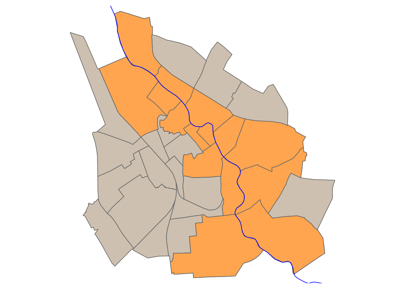
2.4.3. Touching geometry
Geometry is considered touching when two geometries share a common boundary or have at least one point in common without overlapping or intersecting. Touching geometries are typically used to represent features that are physically adjacent or connected, for example, two adjacent polygons on a map may touch along a common boundary.
In R, the st_touches() function is used to determine whether two geometries touch each other. It returns a logical vector indicating which geometries in a dataset touch a specified target geometry.
Let’s identify districts within the districts object that are adjacent to the Taga-Karlova district.
# Filter the "Taga-Karlova" district
tk_dist <- districts %>%
  filter(NIMI == "Taga-Karlova")

# Use st_touches to find districts touching "karlova"
touching_dist <- st_touches(tk_dist, districts, sparse = FALSE)

# Extract district names that touch the "Taga-Karlova" district
touching_dist_names <- districts[touching_dist, ]
Plot the result:
# Plot the intersecting districts
tmap_mode("plot")
tmap mode set to plottingtm_shape(districts) +
tm_polygons(col = "#CDC0B0")+
tm_shape(touching_dist_names) +
tm_polygons(col = "#CD5C5C")+
tm_shape(tk_dist)+
tm_polygons(col = "#7CCD7C") +
tm_layout(frame = FALSE)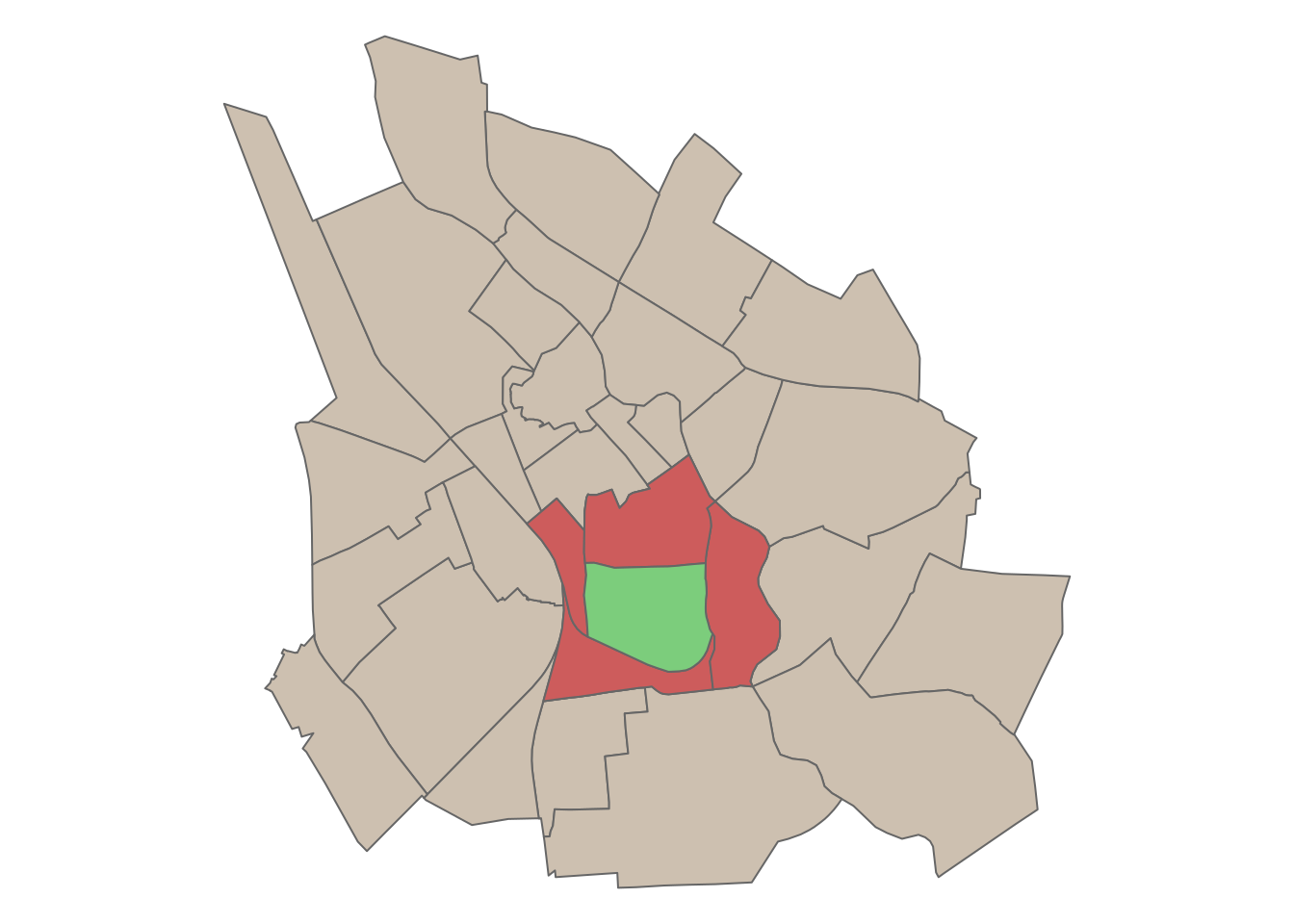
As the last step, let’s save the Emajõgi river (ema_riv_3301) and Tartu shops (shops_new) datasets in our current working directory (R_02 folder) for later use.
# Save the 'ema_riv_3301' object as 'ema_river'
st_write(ema_riv_3301, "ema_river.gpkg",  update = TRUE)  # saves a river as "ema_river.gpkg" file

# Save the 'shops_new' object as 'tartu_shops'
st_write(shops_new, "tartu_shops.gpkg", update = TRUE) # saves the shops as "tartu_shops.gpkg" file