library(terra)      # For working with raster data and spatial analysis
library(sf)         # For handling spatial data and geometry operations
library(tidyverse)  # For data manipulation and visualization
library(tmap)       # For thematic mapping and spatial visualization
library(viridis) # For color maps that are perceptually uniformLesson 5: Raster data analysis
In this lesson, we’ll explore the manipulation of raster data in R. This encompasses tasks such as managing CRSs, extracting values from raster data, cropping, computing zonal statistics, and executing raster algebra operations.
Learning outcomes
At the end of this lesson, the students should be able to:
- Describe what a raster dataset is and its fundamental attributes
- Manage CRSs for raster data
- Extract values from raster data
- Perform zonal statistics and raster calculations
Let’s import all the necessary packages for the lesson.
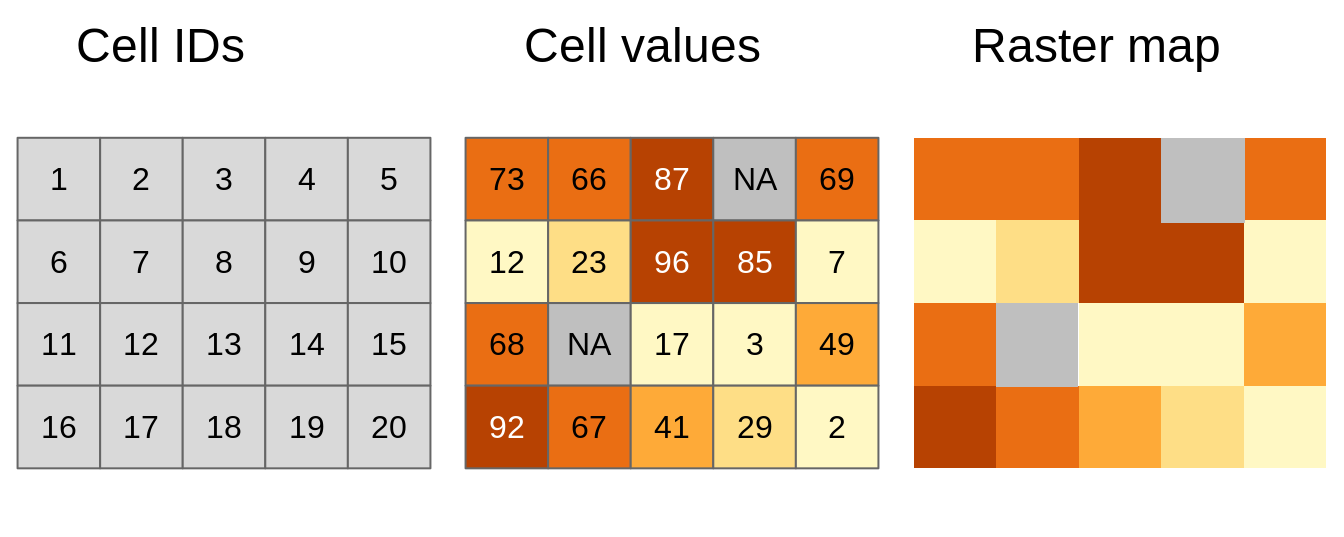
Raster data (aka grid data) is a type of geospatial data representation, where each cell or pixel has a single associated value. Depending on the type of values, we can distinguish continuous and categorical rasters. In continuous rasters, such as elevation or precipitation, values vary progressively. Categorical rasters, on the other hand, uses integer values to represent classes. Their examples include land cover or soil types maps.
A raster can contain single or multiple bands. A single-band raster has one layer of information per pixel, while a multi-band raster has multiple layers, each capturing distinct characteristics. Multi-band rasters are commonly encountered in applications such as satellite imagery, where different bands capture information about various surface features or properties. The figure below provides a fundamental depiction of the raster data model:
Raster data can come in various file formats. Some of the frequently used file formats for raster data include GeoTIFF (.tif), ASCII Grid (.asc), Erdas Imagine (.img), NetCDF (.nc), and ENVI (.hdr). You can find further details about these raster data formats by visiting this link. In this course, we will use the .tif format.
The raster and terra are the most commonly used packages in R for handling spatial raster data. The terra package is relatively newer and was developed as a successor to raster to address some design considerations.
The terra package was designed to overcome the drawbacks of raster packages, particularly issues related to speed and memory when handling large raster datasets. The raster package tends to load the entire dataset into memory, which can be limiting for large datasets. However, the terra is designed to handle out-of-memory processing more efficiently, allowing for the analysis of larger-than-memory datasets. terra also has functionality to work with vector data.
If no output filename is specified to a function, and the output raster is too large to keep in memory, the results are written to a temporary file. terra package has only one object class for raster data, SpatRaster and no distinctions between one-layer and multi-layer rasters is necessary.
Throughout this lesson and the whole course, we will make extensive use of terra package for reading, writing, and manipulating raster data.
5.1. Creating a raster object
To gain a better understanding of raster data, let’s build a raster grid from scratch. A raster object in R can easily be created using the rast() function from terra package. The default settings will create a raster data structure with a geographic CRS (lon/lat WGS 84).
The next code creates a raster object by first defining the spatial extent of the area of interest, and assigning random values to the raster cells using terra package.
# Define the extent
extent <- ext(c(21.82, 28.20, 57.50, 59.67))

# Set a seed for reproducibility
set.seed(1234)

# Create a raster with the custom extent
my_rast <- rast(extent, nrows = 10, ncols = 10)

# Assign random values to the raster cells
values(my_rast) <- runif(ncell(my_rast)) * 100
For quick raster plotting, we can use the built-in plot function:
# Plot the raster
plot(my_rast, col = viridis(13))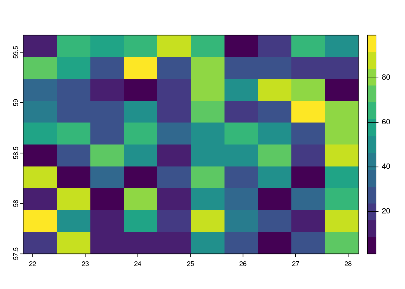
Let’s check the attributes of our raster data:
my_rastclass : SpatRaster
dimensions : 10, 10, 1 (nrow, ncol, nlyr)
resolution : 0.638, 0.217 (x, y)
extent : 21.82, 28.2, 57.5, 59.67 (xmin, xmax, ymin, ymax)
coord. ref. : lon/lat WGS 84
source(s) : memory
name : lyr.1
min value : 0.9495756
max value : 99.2150418 class: the type of the object, in this case aSpatRaster.nrow,ncol: the number of rows and columns in the data (imagine a spreadsheet or a matrix).nlyr: the number of layers in the rasterresolution: the size of each pixel (deg decimal).extent: the spatial extent of the raster. This value will be in the same coordinate units as the crs of the raster.coord. ref: the crs string for the raster. This raster is in Geographical Coordinate system with a datum of WGS 84.
Check the extent of a raster:
ext(my_rast)SpatExtent : 21.82, 28.2, 57.5, 59.67 (xmin, xmax, ymin, ymax)Get some statistics of raster layer:
summary(my_rast) lyr.1
Min. : 0.9496
1st Qu.:19.9980
Median :38.6883
Mean :43.7497
3rd Qu.:66.6687
Max. :99.2150 In this lesson, we will make use of a Digital Elevation Model (DEM) of Estonia acquired from the Estonian Land Board for Spatial Data to conduct basic raster operations. Download this DEM data from this link and save it within folder R_05.
The rast() function from the terra package is used to import raster data. It doesn’t matter if our raster is continuous, discrete, or contains several bands, the rast() function will correctly read and manipulate terra object.
Let’s import the raster data into our current R session:
dem_est <- rast("dem_est.tif")
dem_est
class : SpatRaster
dimensions : 4193, 6270, 1 (nrow, ncol, nlyr)
resolution : 0.001046233, 0.0005308986 (x, y)
extent : 21.68318, 28.24306, 57.47179, 59.69785 (xmin, xmax, ymin, ymax)
coord. ref. : lon/lat WGS 84 (EPSG:4326)
source : dem_est.tif
name : dem_est
min value : -13.41245
max value : 314.34155 5.2. Raster CRSs in R
Raster datasets extend beyond mere grids of values; they serve as geospatial representations of the Earth’s surface. Each cell in a raster corresponds to a specific real-world location, and this correspondence is defined by the CRS. Handling CRS for raster data involves tasks such as retrieval, definition, and reprojection.
To retrieve the raster CRS in R, we can simply use the crs() function from the terra package. It returns the CRS information associated with the raster. Let’s look at how CRSs are stored in dem_est object:
terra::crs(dem_est, proj = TRUE) # proj = TRUE returns only PROJ-string[1] "+proj=longlat +datum=WGS84 +no_defs"Sometimes, we encounter raster data that lacks a CRS, necessitating its assignment. However, it is crucial to ensure certainty regarding the correct CRS before making any assignments.
Often times, we come across raster data without a CRS, requiring us to assign one. However, it is always important to confirm the correct CRS before assigning one.
Similar to vector data (as discussed in lesson 2), we can assign a CRS to raster data using an EPSG code which corresponds to a particular spatial reference system or projection, and it provides a convenient way to reference and communicate information about the coordinate system used to represent geospatial data.
The format for specifying EPSG codes is a bit different when working with rasters. Instead of just a EPSG code, a string must be provided with +init=epsg: preceding the number.
To practice how to assign CRS to a raster object, let’s remove the CRS from dem_est and then set it to the World Geodetic System (WGS84; EPSG:4326):
# Create a copy of 'dem_est' for backup
dem_est1 <- dem_est

# Remove the CRS from 'dem_est1'
crs(dem_est1) <- NULL

#Assign CRS to 'dem_est1'
crs(dem_est1) <- "+init=epsg:4326"
Warning in x@cpp$set_crs(value): GDAL Message 1: +init=epsg:XXXX syntax is
deprecated. It might return a CRS with a non-EPSG compliant axis order.To conduct meaningful spatial operations and analyses, it is important to ensure that spatial datasets share the same CRS. This alignment is typically achieved by reprojecting raster data. Transforming CRS for vector datasets is straightforward, involving the transformation of vertices. However, with raster datasets, the process is more intricate. Reprojecting raster data requires resampling, leading to alterations in the raster’s geometric characteristics and the recomputation of pixel values.
Raster data in R are reprojected using the project() function from the terra package. This process involves resampling values onto a new raster grid within the updated projection. Similar to the st_transform() function, the first argument designates the dataset for reprojection, and the second argument indicates the new CRS.
By default, the project() function uses bilinear interpolation, which is ideal for continuous data like elevation or temperature. However, for categorical data like land cover, where maintaining the original class codes is crucial, it’s necessary to specify method = near for nearest neighbor interpolation.
The following code reprojects the dem_est object into the official CRS of Estonia (EPSG:3301):
# Reproject the raster to EPSG:3301
dem_est_proj <- project(dem_est, "+init=epsg:3301", method = "bilinear")

# Retrieve and print the CRS information with projection details
terra::crs(dem_est_proj, proj = TRUE)
[1] "+proj=lcc +lat_0=57.5175539305556 +lon_0=24 +lat_1=59.3333333333333 +lat_2=58 +x_0=500000 +y_0=6375000 +ellps=GRS80 +units=m +no_defs"5.3. Extract raster values
In the previous lessons, we’ve seen how to extract information from vector data sets using spatial joins and queries. The same approach can also be applied on raster data to get the values of raster cells for specific geographic locations or area. You can use points, lines, polygons or an Extent (rectangle) objects.
The extract() function from the terra package is used to extract raster values. Raster value extraction is frequently employed in gathering climate-related information such as temperature and precipitation from satellite imagery and to obtain elevation data from DEMs at specific geographical points. In this tutorial, we will learn how to extract elevation values across Estonia using geographical points associated with Estonian weather stations.
Download the Estonian weather data using this link, obtained from Estonina Weather Service.
# Import weather data
weather_stations <-  read.csv("est_weather.csv")

# Check the result
glimpse(weather_stations)
Rows: 155
Columns: 19
$ name <chr> "Kuressaare linn", "Tallinn-Harku", "Pakri", "Kunda"…
$ wmocode <int> NA, 26038, 26029, 26045, 26046, 26058, 26141, 26145,…
$ longitude <dbl> 22.48944, 24.60289, 24.04008, 26.54140, 27.39827, 28…
$ latitude <dbl> 58.26417, 59.39812, 59.38950, 59.52141, 59.32902, 59…
$ phenomenon <chr> "", "Few clouds", "", "", "", "", "", "", "", "Overc…
$ visibility <dbl> NA, 35, 35, 50, 20, 20, 20, 20, 20, 35, 20, 35, 20, …
$ precipitations <dbl> NA, 0, 0, 0, 0, 0, 0, 0, 0, 0, 0, 0, 0, 0, 0, 0, 0, …
$ airpressure <dbl> NA, 1018.1, 1017.6, 1018.3, 1018.6, 1018.6, 1017.9, …
$ relativehumidity <int> 84, 79, 73, 61, 77, 86, 75, 80, 86, 78, 90, 88, 88, …
$ airtemperature <dbl> 1.9, 3.0, 3.4, 4.2, 1.9, 1.7, 1.6, 2.9, 0.7, 1.7, 1.…
$ winddirection <int> NA, 90, 89, 89, 69, 50, 81, NA, 52, 80, 46, 64, 56, …
$ windspeed <dbl> NA, 4.1, 5.8, 12.0, 4.9, 5.7, 6.9, NA, 5.1, 4.0, 4.6…
$ windspeedmax <dbl> NA, 7.6, 11.9, 15.7, 7.8, 8.7, 11.1, NA, 8.8, 8.7, 8…
$ waterlevel <int> NA, NA, NA, NA, NA, NA, NA, NA, 64, NA, NA, NA, NA, …
$ waterlevel_eh2000 <int> NA, NA, NA, 25, NA, NA, NA, NA, NA, NA, NA, NA, NA, …
$ watertemperature <dbl> NA, NA, NA, 7.800, NA, NA, NA, NA, NA, NA, NA, NA, N…
$ uvindex <dbl> NA, 0.7, NA, NA, NA, NA, NA, NA, NA, NA, NA, NA, NA,…
$ sunshineduration <int> NA, 82, NA, NA, 130, NA, NA, 51, 59, 19, 0, NA, 7, N…
$ globalradiation <int> NA, 82, NA, NA, NA, 130, NA, 67, NA, 74, NA, NA, NA,…Our weather stations data is stored as a data frame object, while the elevation data from which we aim to extract elevation values is in spatial (raster) format. Consequently, it becomes necessary to convert the data frame into spatial (vector) object. Once this transformation is complete, utilizing the vector/sf object representing our station points, we can proceed to extract elevation values from the dem_est object we created above.
#Clean up the data by selecting
weather_stations_df <- weather_stations %>%
  select(latitude, longitude, airtemperature)

# Create simple feature for weather object
weather_stations_sf <- st_as_sf(weather_stations_df,
                                coords = c("longitude", "latitude"), crs = 4326)

# Check the result
glimpse(weather_stations_sf)
Rows: 155
Columns: 2
$ airtemperature <dbl> 1.9, 3.0, 3.4, 4.2, 1.9, 1.7, 1.6, 2.9, 0.7, 1.7, 1.6, …
$ geometry <POINT [°]> POINT (22.48944 58.26417), POINT (24.60289 59.398…Let’s create a plot that displays the station together with the DEM data:
# Create a combined plot
tm_shape(dem_est) +
  tm_raster(palette = terrain.colors(8),
            title = "Elevation (m)",
            alpha=.8,
            style="cont") +
  tm_shape(weather_stations_sf)+
  tm_dots(col = "red", size = 0.2, alpha=.5) +
  tm_graticules(lines = FALSE)
stars object downsampled to 1223 by 818 cells. See tm_shape manual (argument raster.downsample)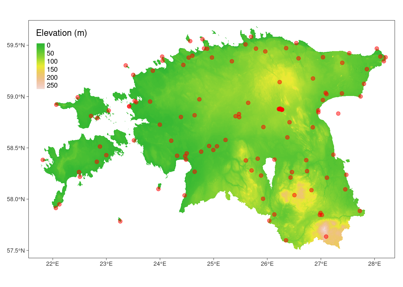
Now, let’s proceed with extracting the elevation values for each weather stations point, which results in a data frame with column names ID (the row number of the stations)
# Extract elevation values at station points
elev_values <- terra::extract(dem_est, weather_stations_sf)

# Add elevation_values to weather_stations_df object
stations_sf_elev <- weather_stations_sf %>%
  mutate(elev = elev_values$dem_est)

# Check if "stations_sf_elev" contains any missing values
anyNA(stations_sf_elev)
[1] TRUE# For certain coastal stations, the elevation values shows NA. It can be assumed that the elevation for these stations is relatively close to zero.
stations_sf_elev$elev[is.na(stations_sf_elev$elev)] <- 0
# check the result
glimpse(stations_sf_elev)Rows: 155
Columns: 3
$ airtemperature <dbl> 1.9, 3.0, 3.4, 4.2, 1.9, 1.7, 1.6, 2.9, 0.7, 1.7, 1.6, …
$ geometry <POINT [°]> POINT (22.48944 58.26417), POINT (24.60289 59.398…
$ elev <dbl> 5.087852, 32.220737, 22.995630, 2.388902, 72.981567, 28…Let’s create a plot using tmap to visualize the extracted data.
# Create a tmap plot for elevation data
tm_shape(dem_est) +
  tm_raster(palette = terrain.colors(8),
            alpha = .7,
            legend.show = FALSE)+
  tm_shape(stations_sf_elev) +
  tm_bubbles(size = "elev",
             col = "red",
             shape = 16,
             alpha=.6,
             title.size = "Elevation (m)") +
   tm_layout(legend.position = c("left", "bottom")) +
  tm_graticules(lines = FALSE)
stars object downsampled to 1223 by 818 cells. See tm_shape manual (argument raster.downsample)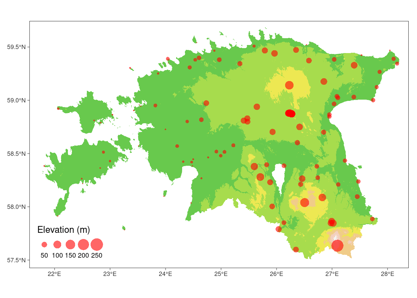
5.4. Raster cropping
Many geographic data projects involve integrating data from many different sources, such as remote sensing images (rasters) and administrative boundaries (vectors). Often the extent of input raster datasets is larger than the area of interest. In this case, raster cropping and masking are useful for unifying the spatial extent of input data.
Cropping rasters in R is pretty straightforward using the crop() function from terra package. The function reduces the rectangular extent of the object passed to its first argument based on the extent of the object passed to its second argument.
In this lesson, we will crop our dem_est_proj raster using the geographic extent of the Porijôgi catchment, which you are familiar with from python course. Please download Porijôgi catchment data using this link.
Let’s import the pori_landuse data and creating a joint visualization with the raster data:
# Import Porijõgi catchment
pori <- st_read("pori_landuse.gpkg")
Reading layer `pori_landuse' from data source
`/home/geoadmin/dev/simply-general/teaching/geospatial_python_and_r/R_05/pori_landuse.gpkg'
using driver `GPKG'
Simple feature collection with 62 features and 1 field
Geometry type: MULTIPOLYGON
Dimension: XY
Bounding box: xmin: 649914 ymin: 6445252 xmax: 669491.9 ymax: 6462773
Projected CRS: Estonian Coordinate System of 1997# Plot
tm_shape(dem_est_proj) +
tm_raster(palette = terrain.colors(8),
title = "Elevation (m)",
alpha = 0.8,
style = "cont") +
tm_shape(st_union(pori)) +
tm_borders(lwd = 2, col = "red") +
tm_graticules(lines = FALSE)stars object downsampled to 1241 by 806 cells. See tm_shape manual (argument raster.downsample)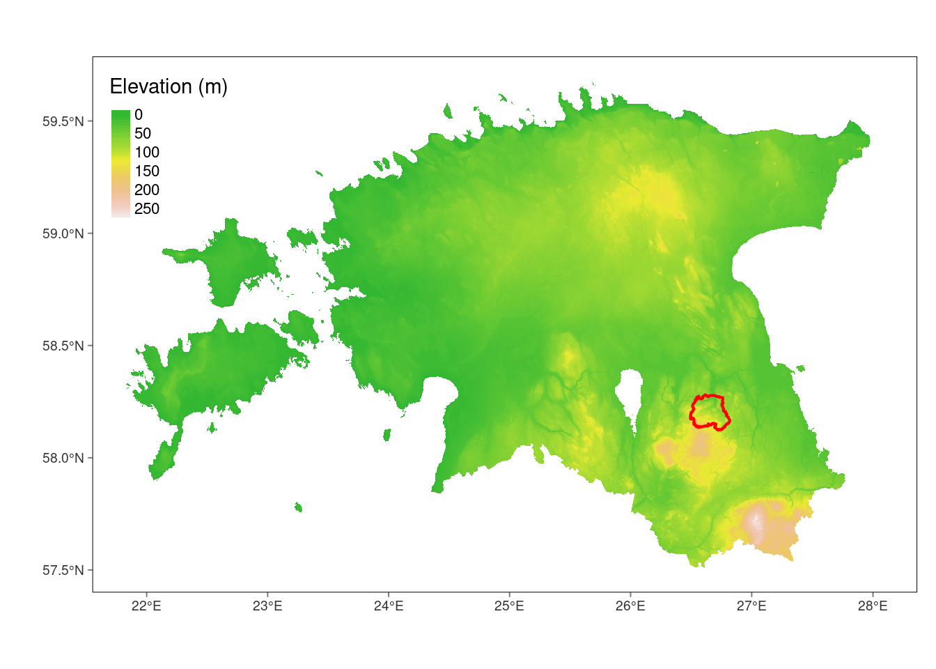
Everything looks great! Let’s move forward with the cropping process. The next code crops the DEM of Estonia to the extent of the Porijôgi catchment.
# Crop the raster based on the extent of the Porijôgi layer
pori_dem_crop <- crop(dem_est_proj, pori)

# Plot cropped dem
tm_shape(pori_dem_crop) +
  tm_raster(palette = terrain.colors(8),
            title = "Elevation (m)",
            alpha = 0.8, style = "cont") +
  tm_layout(legend.show = FALSE) +
  tm_shape(st_union(pori)) +
  tm_borders(lwd = 2, col = "red") +
  tm_graticules(lines = FALSE)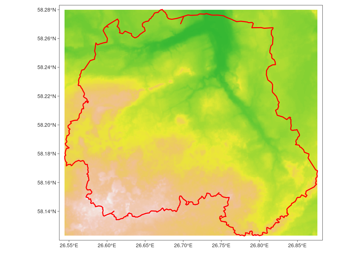
Crop returns a geographic subset of an object as specified by an extent object (or object from which an extent object can be extracted/created), not to the actual boundaries of the catchment. To do that, we have to add one more step using mask() function.
#mask pori catchment
pori_dem_mask <- mask(pori_dem_crop, pori)
Warning: [mask] CRS do not match# Plot cropped dem
tm_shape(pori_dem_mask) +
tm_raster(palette = terrain.colors(8),
alpha = 0.8, style = "cont") +
tm_layout(legend.show = FALSE) +
tm_shape(st_geometry(pori)) +
tm_borders() +
tm_graticules(lines = FALSE)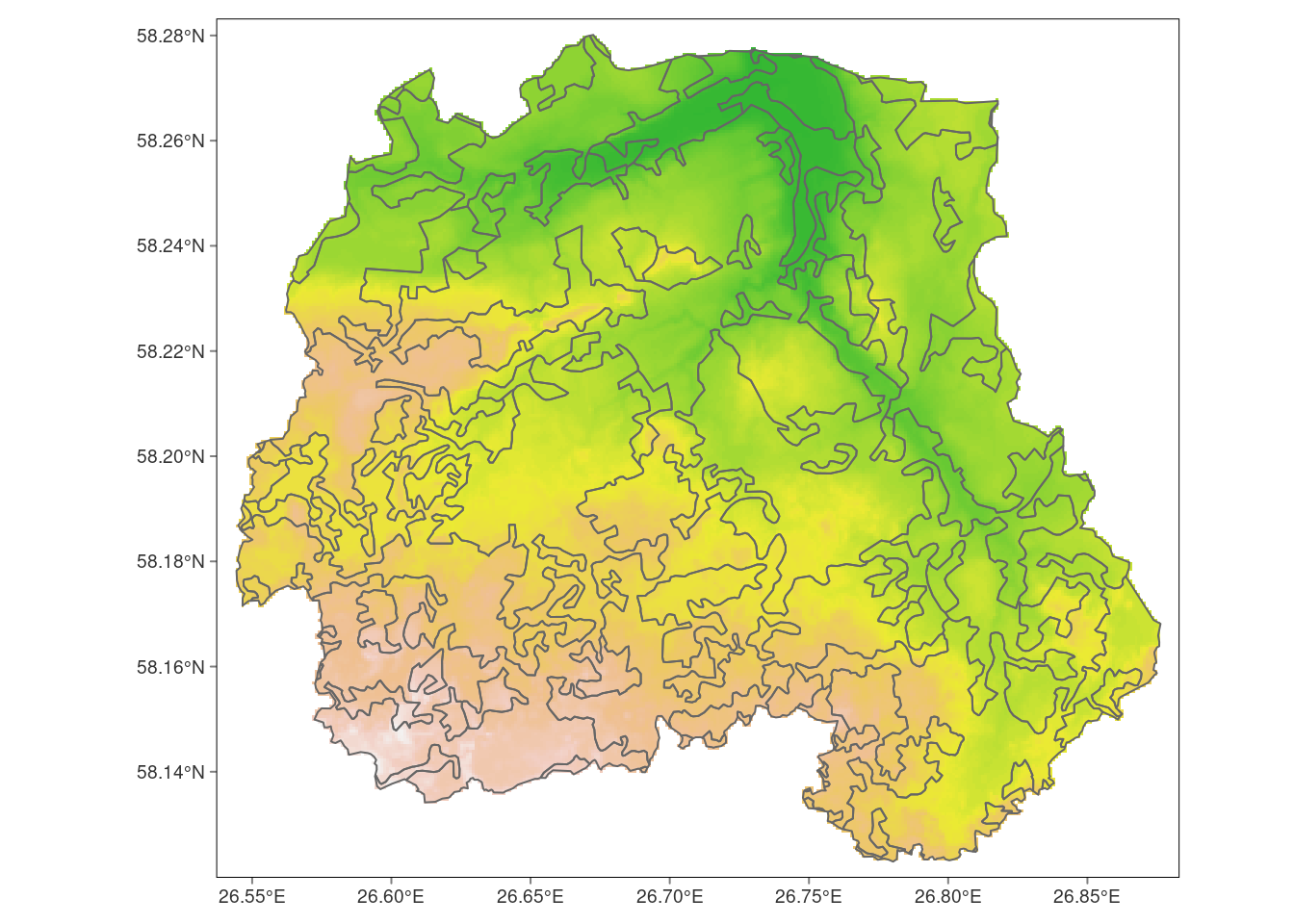
5.5. Zonal statistics
Zonal statistics refer to the process of extracting statistical information from raster data within predefined zones, for example, polygons from a vector layer. Summary data obtained through zonal statistics include mean, median, count, standard deviation, and sum. Zonal statistics summarize the values of a particular group of cells. Calculating zonal statistics involves overlaying the vector zones on the raster, and for each zone, computing the desired statistics from the values of the intersecting raster cells.
In R, calculating zonal statistics can be achieved by using the extract() function from the terra package. In this tutorial, we’ll extract the DEM cell values in the pori_dem_mask object that are within the land-use zones of Porijôgi catchment (mean elevation for each of 62 polygons in the pori object).
# Calculate zonal statistics
mean_elev <- terra::extract(pori_dem_mask, pori, fun = mean)
Warning: [extract] transforming vector data to the CRS of the raster# Add the extracted elevation to pori object
pori_elev <- pori %>%
mutate(elev = mean_elev$dem_est)
# Check the output
slice(pori_elev, 15:25)Simple feature collection with 11 features and 2 fields
Geometry type: MULTIPOLYGON
Dimension: XY
Bounding box: xmin: 650371.4 ymin: 6446575 xmax: 669087.9 ymax: 6462345
Projected CRS: Estonian Coordinate System of 1997
First 10 features:
landuse elev geom
1 cropland 74.56572 MULTIPOLYGON (((661788.7 64...
2 cropland 100.14195 MULTIPOLYGON (((666725.5 64...
3 cropland 94.67468 MULTIPOLYGON (((668155.1 64...
4 cropland 84.73435 MULTIPOLYGON (((667429.6 64...
5 cropland 98.44496 MULTIPOLYGON (((668552.2 64...
6 water 106.61952 MULTIPOLYGON (((651615.6 64...
7 grasslands 152.50988 MULTIPOLYGON (((655040.5 64...
8 grasslands 142.56590 MULTIPOLYGON (((658480.6 64...
9 grasslands 86.82963 MULTIPOLYGON (((658497 6454...
10 grasslands 87.05816 MULTIPOLYGON (((655808.6 64...Let’s visualize the land-use and its corresponding average elevation:
# Create a map
tm_shape(pori) +
  tm_polygons(col = "landuse",
              alpha = 0.7,
              title = "Land use") +
  tm_shape(pori_elev)+
  tm_symbols(col = "elev",
             palette = "Reds",
             style = "cont",
             title.col = "Elevation (m)") +
  tm_layout(legend.outside = TRUE)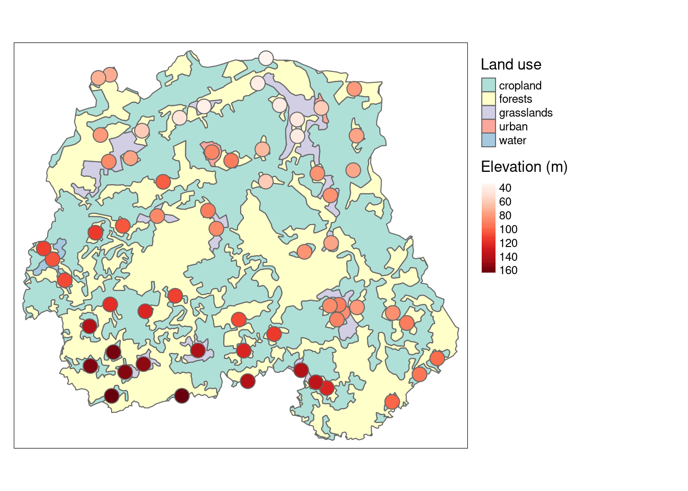
5.6. Raster Calculations
Raster calculations, also known as raster algebra or map algebra, involve performing mathematical or logical operations on raster datasets. These operations allow you to create new raster layers by combining or modifying the values of existing raster layers. Raster calculations are common in GIS and remote sensing analysis for tasks such as map manipulation, modeling, and spatial analysis.
In this tutorial, we will employ the raster calculation method to investigate the impact of elevation and coordinate values on air temperature in Estonia. The analysis will involve utilizing raster algebra in conjunction with a linear regression model, utilizing the stations_sf_elev object established earlier.
Let’s start the process by preparing the elevation and coordinate data essential for our model:
# Extract X and Y values from the stations_sf_elev object
air_temp_coord <- stations_sf_elev %>%
  st_coordinates()

# Combine "stations_sf_elev" and "air_temp_coord" objects
air_temp_sf <- bind_cols(stations_sf_elev, air_temp_coord)

# Convert "air_temp_sf" to dataframe
air_temp_df <- air_temp_sf %>%
  st_drop_geometry()

# Display the resulting dataframe
slice(air_temp_df, 1:10)
airtemperature elev X Y
1 1.9 5.087852 22.48944 58.26417
2 3.0 32.220737 24.60289 59.39812
3 3.4 22.995630 24.04008 59.38950
4 4.2 2.388902 26.54140 59.52141
5 1.9 72.981567 27.39827 59.32902
6 1.7 28.599640 28.10933 59.38953
7 1.6 120.833504 26.23074 59.14135
8 2.9 32.596046 26.95211 58.86540
9 0.7 70.286453 26.41501 58.74984
10 1.7 69.421394 26.46131 58.26407Let’s check if there is a correlation between air temperature and both the coordinates and elevation using the ggplot2 package to create a scatter plot with a linear regression line:
#Check the correlation between airtemperature and longitude
ggplot(data = air_temp_df)+
  geom_point(aes(x= X, y = airtemperature))+
  stat_smooth(aes(x= X, y = airtemperature), method = "lm")
`geom_smooth()` using formula = 'y ~ x'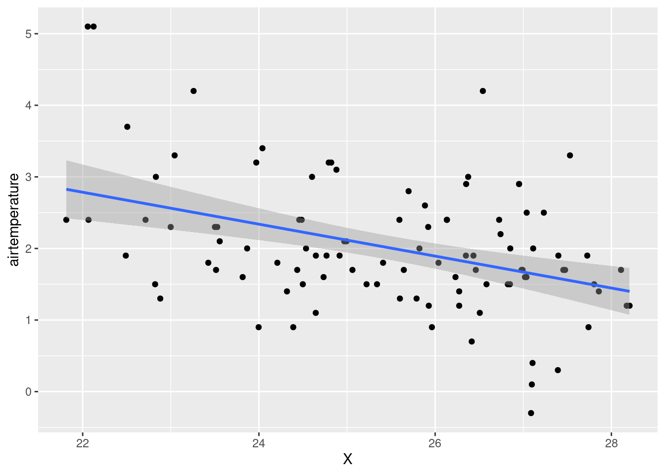
#Check the correlation between airtemperature and latitude
ggplot(data = air_temp_df)+
  geom_point(aes(x= Y, y = airtemperature))+
  stat_smooth(aes(x= Y, y = airtemperature), method = "lm")
`geom_smooth()` using formula = 'y ~ x'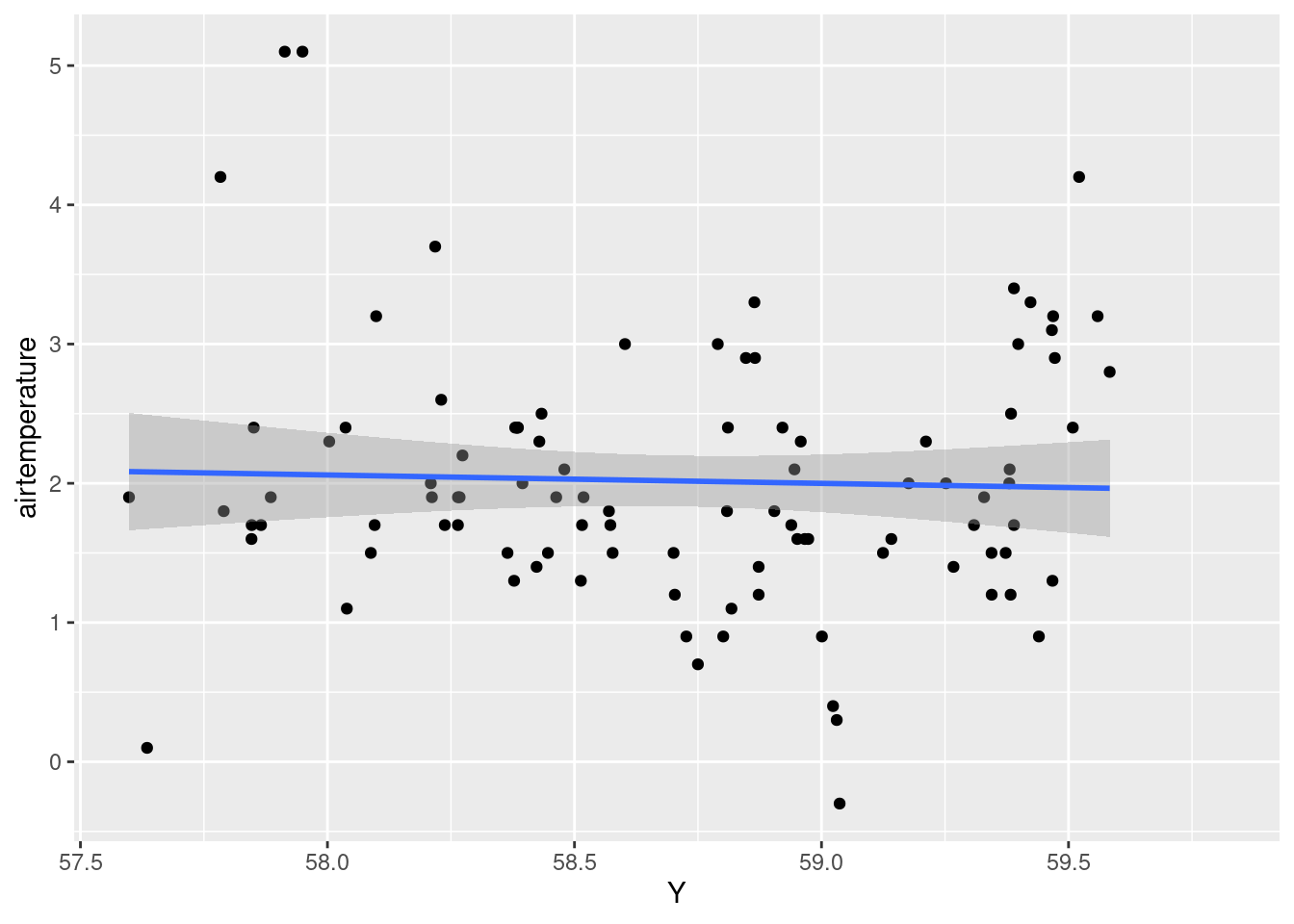
#Check the correlation between airtemperature and elevation
ggplot(data = air_temp_df)+
  geom_point(aes(x= elev, y = airtemperature))+
  stat_smooth(aes(x= elev, y = airtemperature), method = "lm")
`geom_smooth()` using formula = 'y ~ x'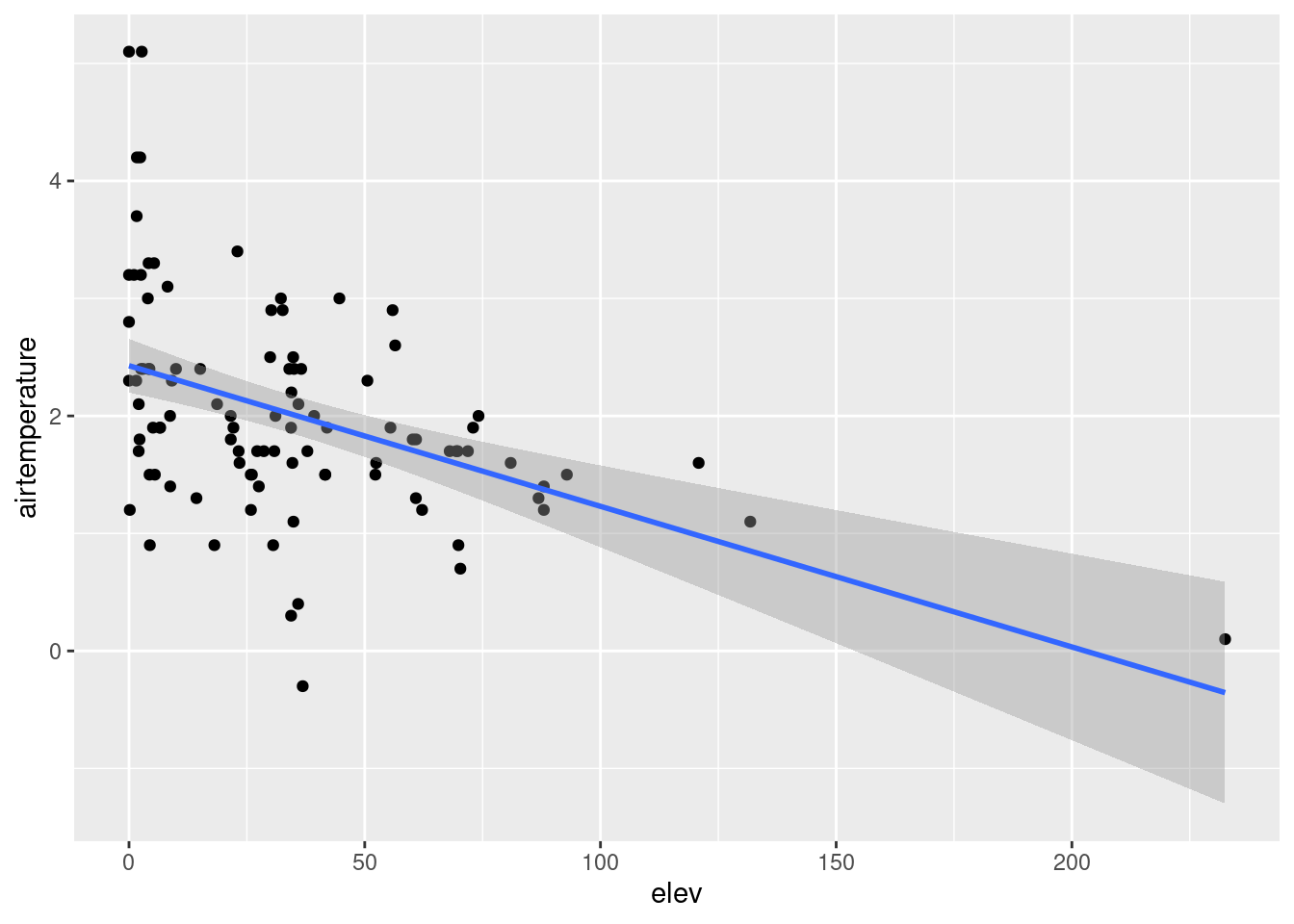
Using a linear regression model, we can investigate the correlation between air temperature (dependent variable) and the independent variables, which include coordinates and elevation. This approach allows us to gain further insights into the relationships and potential influences of these factors on airtemperature.
#Fit a linear regression model
airtemperature_lm <- lm(formula = airtemperature ~ X + Y + elev, data = air_temp_df)

#Model summary
summary(airtemperature_lm)
Call:
lm(formula = airtemperature ~ X + Y + elev, data = air_temp_df)

Residuals:
     Min       1Q   Median       3Q      Max
-2.04656 -0.43139 -0.09671  0.43421  2.24944

Coefficients:
             Estimate Std. Error t value Pr(>|t|)
(Intercept) 14.702569   9.050945   1.624 0.107564
X           -0.117652   0.057382  -2.050 0.043059 *
Y           -0.159383   0.157676  -1.011 0.314642
elev        -0.009759   0.002773  -3.519 0.000664 ***
---
Signif. codes:  0 '***' 0.001 '**' 0.01 '*' 0.05 '.' 0.1 ' ' 1

Residual standard error: 0.8009 on 96 degrees of freedom
  (55 observations deleted due to missingness)
Multiple R-squared:  0.258, Adjusted R-squared:  0.2348
F-statistic: 11.12 on 3 and 96 DF,  p-value: 2.482e-06
Here’s a concise summary of the linear regression model output:
The coefficient for
longitude(-0.117652) suggests that a one-unit increase in longitude is associated with a predicted decrease of approximately 0.117652 units in air temperature, and this effect is highly significant atp = 0.043059.The coefficient for
latitude(-0.159383) suggests that a one-unit increase inlatitudeimplies a predicted decrease of about0.159383units, but the effect is not statistically significant atp = 0.314642.The coefficient for
elevation(-0.009759) suggests that a one-unit increase in elevation is associated with a predicted decrease of approximately 0.009759 units, and this effect is highly significant atp = 0.000664.
Let’s exclude latitude from the analysis due to its statistically insignificant impact on air temperature and use the longitude and elevation variables in the linear regression model coefficients (airtemperature_lm) to predict air temperature (air_temp_mod).
# Predict airtemperature (air_temp_mod) and add to air_temp_sf object
air_temp_sf <- air_temp_sf %>%
  mutate(air_temp_mod =
           X * coef(airtemperature_lm)[2] +
           elev * coef(airtemperature_lm)[4] +
           coef(airtemperature_lm)[1])

#prediction result
glimpse(air_temp_sf)
Rows: 155
Columns: 6
$ airtemperature <dbl> 1.9, 3.0, 3.4, 4.2, 1.9, 1.7, 1.6, 2.9, 0.7, 1.7, 1.6, …
$ elev <dbl> 5.087852, 32.220737, 22.995630, 2.388902, 72.981567, 28…
$ X <dbl> 22.48944, 24.60289, 24.04008, 26.54140, 27.39827, 28.10…
$ Y <dbl> 58.26417, 59.39812, 59.38950, 59.52141, 59.32902, 59.38…
$ geometry <POINT [°]> POINT (22.48944 58.26417), POINT (24.60289 59.398…
$ air_temp_mod <dbl> 12.00699, 11.49354, 11.64979, 11.55661, 10.76687, 11.11…Let’s create a visualization for final result that illustrates how geographical coordinates and elevation impact air temperature:
#Plot
tm_shape(dem_est)+
  tm_raster(palette = terrain.colors(8), alpha = .7, legend.show = FALSE) +
  tm_shape(air_temp_sf) +
  tm_dots(col = "air_temp_mod", size = 0.5, shape = 19, style = "cont",
          title = "Air temperature (°C)") +
  tm_graticules(lines = FALSE)
stars object downsampled to 1223 by 818 cells. See tm_shape manual (argument raster.downsample)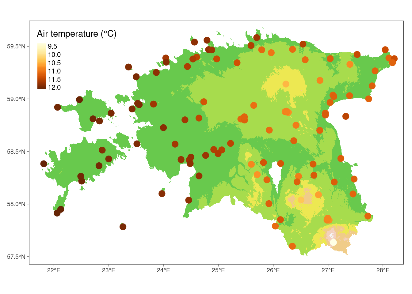
5.7. Remote sensing in R
Remote sensing entails the manipulation of multiband raster data, with each spectral band capturing information from specific segments of the electromagnetic spectrum. These bands, commonly acquired through sensors on satellites or other platforms, provide a comprehensive perspective on the Earth’s surface.
In this section, we’ll explore the basics of remote sensing analysis in R. We will focus on basic tasks like importing multiband images, generating image composites, and computing specific spectral indices, without delving into details.
To illustrate these techniques, we’ll be using a Landsat 8 scene from 22/Sep/2023 of the Tartu region, Estonia. The data can be freely obtained from the USGS repositories using the Earth Explorer data discovery tool.
Download the Landsat 8 images using this link. The Landsat 8 data comes as a collection eleven bands; plus a quality band. However, to keep things neat, we have chosen only spectral bands 1-7. Save the downloaded file to your current working directory, and then unzip and import the files using the following code.
# Specify the path to the zip file
zipped_file_path <- "D:/teaching/rgeospatial_ut/R_05/landsat8.zip"  #Please replace this with the path to your zip file path

# Read and unzip the file
unzip(zipped_file_path, exdir = "D:/teaching/rgeospatial_ut/R_05/") # Make sure to replace this with the desired extraction directory
Warning in unzip(zipped_file_path, exdir = "D:/teaching/rgeospatial_ut/R_05/"):
error 1 in extracting from zip file# Read the bands into a raster stack and assign custom names
ls <- terra::rast(paste0("Ls8_b", 1:7, ".tif"))
names(ls) <- c("Coastal","Blue","Green","Red","NIR","SWIR-1","SWIR-2")
# Check what is inside
ls #7 bandas, 30m resolutionclass : SpatRaster
dimensions : 568, 987, 7 (nrow, ncol, nlyr)
resolution : 30, 30 (x, y)
extent : 470385, 499995, 6461355, 6478395 (xmin, xmax, ymin, ymax)
coord. ref. : WGS 84 / UTM zone 35N (EPSG:32635)
sources : Ls8_b1.tif
Ls8_b2.tif
Ls8_b3.tif
... and 4 more source(s)
names : Coastal, Blue, Green, Red, NIR, SWIR-1, ... Let’s plot spectral bands from 2-4 only:
plot(ls[[c(2,3,4,5)]], col = gray(0:100/100, alpha = 0.8))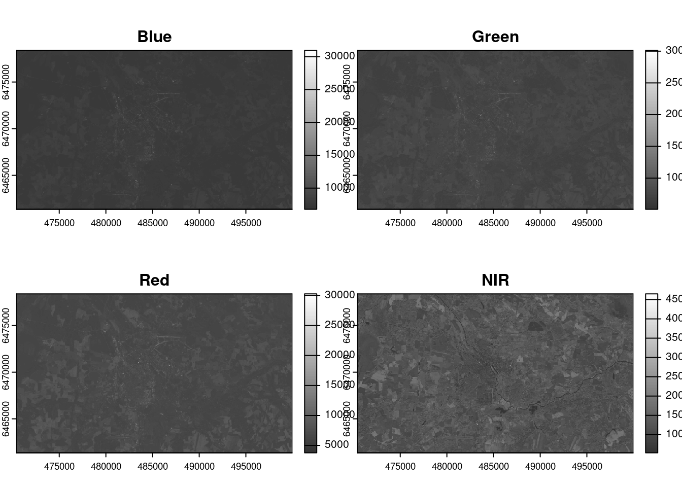
#In R, double square brackets ([[ ]]) are used for extracting elements from a list by indexing,  to access specific layers within the list, in our case.
#A single square bracket "[ ]" is used for subsetting lists, but when you want to extract the actual contents of an element within the list (rather than a sublist), you use double square brackets "[[ ]]".

# "grey(0:100)" generates a grayscale color palette with shades ranging from black (0) to white (100). "/100" normalizes these integers to a range of 0 to 1.
Each band represent how much incident solar radiation is reflected for a particular wavelength range. For example, vegetation reflects more energy in NIR (B5) than other wavelengths and thus appears brighter. In contrast, water absorbs most of the energy in the NIR wavelength and it appears dark.
We do not gain that much information from these grey-scale plots; they are often combined into a composite (e.g, true or false color) to create more interesting plots.
To make a true (or natural) color image, we need bands in the red, green and blue regions. For our current Landsat image, band 4 (red), 3 (green), and 2 (blue) can be used. Another popular image visualization method in remote sensing is known false color image in which NIR, red, and green bands are combined. This representation is popular as it makes easy to see the vegetation (in red).
The plotRGB() function from terra package can be used to visualize the composite images. We can also supply additional arguments to plotRGB to improve the visualization (e.g. a linear stretch of the values, using strecth = "lin").
Let’s generate both a true color composite and a false color composite plots:
#True color composite
plotRGB(ls, r = 4, g = 3, b = 2, stretch = "lin",
        main = "True Color Composite")
#False color composite
plotRGB(ls, r = 5, g = 4, b = 3, stretch = "lin",
        main = "False Color Composite")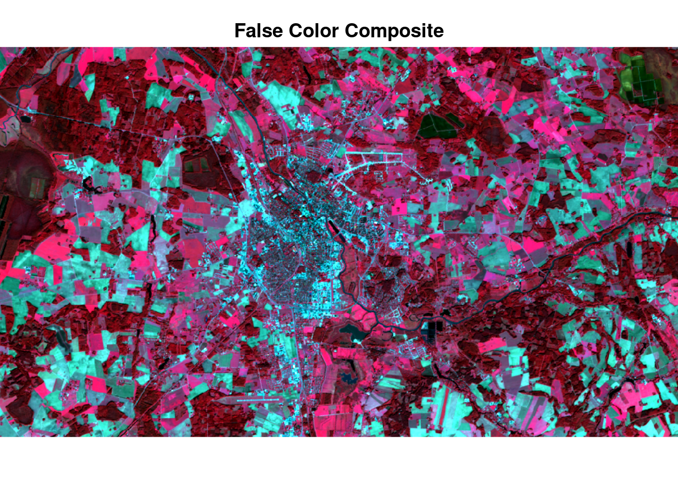
We can now move forward with the computation of Normalized Difference Vegetation Index (NDVI) and Soil Adjusted Vegetation Index (SAVI) using raster calculation operations.
The NDVI is an index of plant greenness or photosynthetic activity, and is one of the most commonly used vegetation indices. Vegetation indices are based on the observation that different surfaces reflect different types of light differently. Vegetation that is dead or stressed reflects more red light and less near infrared light.
NDVI is calculated as: NDVI = (NIR - RED)/(NIR +RED)
# Calculate NDVI
NDVI <- (ls[[5]] - ls[[4]]) / (ls[[5]] + ls[[4]])
names(NDVI) <- "NDVI"  # change the name of the layer from "NIR" to "NDVI

# Plot NDVI
plot(NDVI, col = rev(terrain.colors(30)), #rev() function reverses the order of the color
     main = "Normalized Difference Vegetation Index (NDVI)")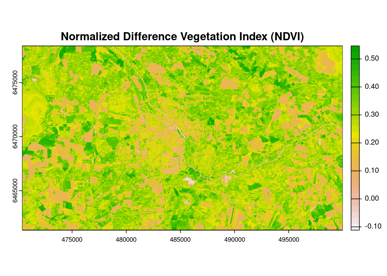
We can explore the distribution of values contained within our raster using the hist() function which produces a histogram. Histograms are often useful in identifying outliers and bad data values in our raster data.
# view histogram of data
hist(NDVI,
     main = "Distribution of NDVI values",
     xlab = "NDVI",
     ylab = "Number of Pixels",
     col = "springgreen")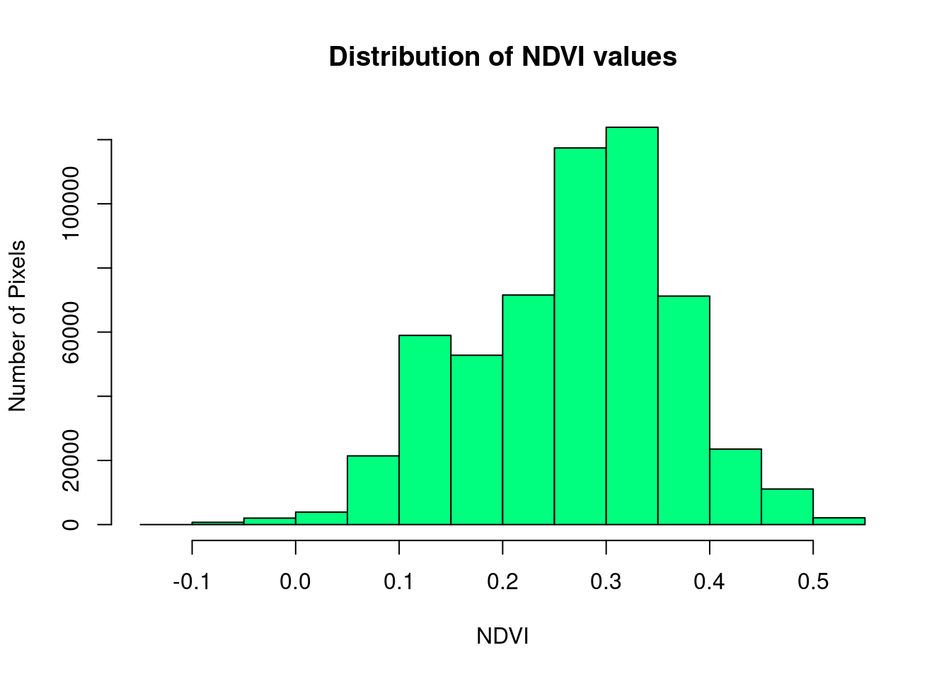
The SAVI index is similar to NDVI, but it suppresses the effects of pixels containing bare soil, by incorporating a canopy background adjustment factor, L, into the calculations. L is a function of vegetation density, which can be based on prior knowledge of vegetation amounts. In the absence of such knowledge, Huete (1988) suggests using a value of L = 0.5 to account for first-order soil background variations. This index is best used in areas with relatively sparse vegetation where soil is visible through the canopy.
SAVI is calculated as: SAVI = (1 + L) x (NIR - RED)/(NIR + RED + L)
# Calculate SAVI
L=0.5
SAVI <- (1 + L) * (ls[[5]] - ls[[4]])/(ls[[5]] + ls[[4]] + L)

# Plot SAVI
plot(SAVI, col = rev(terrain.colors(30)),
     main = "Soil Adjusted Vegetation Index (SAVI)")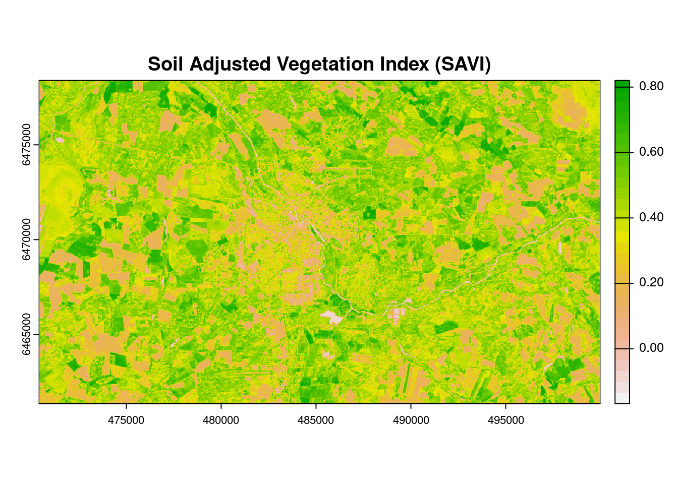
Upon completing raster data processing tasks, exporting the output becomes necessary to ensure the accessibility, shareability, and usability of raster data across various platforms and tools. In R, the terra package provides a convenient and flexible way to export raster objects using writeRaster() function. This function allows users to save raster datasets in various formats, such as GeoTIFF, NetCDF, and others.
Let’s export the NDVI result as a TIFF file.
writeRaster(NDVI, "NDVI.tif", gdal=c("COMPRESS=LZW"), overwrite = TRUE)
#gdal = c("COMPRESS=LZW"): This part specifies GDAL (Geospatial Data Abstraction Library) options for compression.
#It's set to use LZW compression, which is a lossless compression method
5.8. Rasterization
Rasterization is the conversion of vector objects into their representation in raster objects. This process is valuable for simplifying datasets, as it ensures uniform spatial resolution in the resulting raster. Essentially, rasterization functions as a specialized form of geographic data aggregation.
The terra package incorporates the rasterize() function for executing rasterization tasks in R. The primary parameters for this function are the vector object to be rasterized and the template raster object that defines the output’s extent, resolution, and CRS. The template raster can either be an existing valid raster or an empty raster with no cell values. The outcome of rasterization is influenced not only by the characteristics of the template raster but also by the input vector type (e.g., points, polygons) and various arguments provided to the rasterize() function.
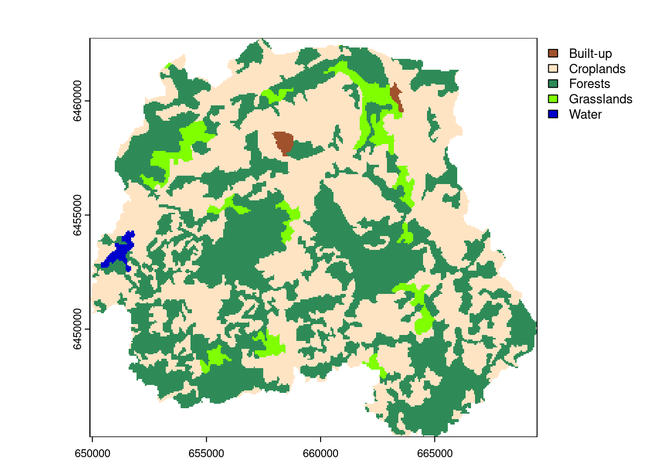
To illustrate the rasterization process, we will apply it to vector data representing land use in the Porijôgi catchment (pori). The DEM raster (pori_dem_mask) will serve as the template for this specific rasterization task.
# Rename land use classes before rasterization
landuse_rename <- c("cropland" = "Croplands",
                    "forests" = "Forests",
                    "grasslands" = "Grasslands",
                    "urban" = "Built-up",
                    "water" = "Water")
# Update a landuse variable in the pori_new dataset by applying a transformation based on the landuse_rename lookup.
pori_new <- pori %>%
  mutate(landuse = landuse_rename[landuse])

# Create a raster template
template <- pori_dem_mask

# Rasterize the landuse data
pori_rast <- rasterize(pori_new, template, field = "landuse")
pori_rast
class : SpatRaster
dimensions : 290, 325, 1 (nrow, ncol, nlyr)
resolution : 60.28752, 60.28752 (x, y)
extent : 649893, 669486.4, 6445273, 6462757 (xmin, xmax, ymin, ymax)
coord. ref. : Estonian Coordinate System of 1997
source(s) : memory
categories : landuse
name : landuse
min value : Built-up
max value : Water Plot the rasterized object:
#Plot
plot(pori_rast, col= c("#A0522D", "#FFE4C4", "#2E8B57", "#7FFF00",  "#0000CD"))