Lesson 8: 3D mapping

Learning outcomes

In this tutorial, we will learn how to create 3D maps in R using the rayshader package. We will use high resolution elevation and Orthophoto datasets specific to the Rummu Quarry area. The tutorial materials have been adapted from the works of Anto Aasa and the code has been adjusted using resources available on the official rayshader site.

At the end of this lesson, the students should be able to:

• Comprehend the features and functionalities of the rayshader package.
• Generate 3D visualizations for spatial data utilizing the rayshader package.
• Transform ggplot visualizations into 3D representations.

Let’s start with installing and loading the packages required for the lesson:

library(rayshader) # For 3D visualizations
library(tidyverse) # For data manipulation and visualization
library(viridis)   # For color scales
library(terra)     # For spatial data manipulation
library(sf)        # For working with simple features 
library(av)        # For handling audio and video files 
# devtools::install_github("mccarthy-m-g/embedr")
library(embedr)    # For embedding content
library(rgl)       # For interactive 3D visualizations

8.1. Introduction

3D mapping is the process of creating three-dimensional representations of objects, surfaces, landscapes, or environments in the digital or physical world. It involves capturing and modeling spatial data to depict objects and terrain in three dimensions, allowing for a more accurate and realistic portrayal compared to traditional 2D mapping methods.It allows for in-depth data analysis and effective communication of complex information, with options for interactivity and customization to enhance the visual appeal and clarity of the plots.

To generate 3D maps in R, various libraries and packages can be used. In this tutorial, we will use the rayshader package, an open-source tool designed for creating both 2D and 3D data visualizations in R. The rayshader uses elevation data in a base R matrix and a combination of raytracing, hillshading algorithms, and overlays to generate stunning 2D and 3D maps. In addition to maps, rayshader also allows the user to translate ggplot2 objects into beautiful 3D data visualizations.

The rayshader package encompasses various essential functions for generating customized 3D visualizations, including:

• raster_to_matrix(): converts a raster objects into a matrix.
• sphere_shade(): maps an RGB texture to a hillshade by spherical mapping.
• render_highquality(): combines the ability to render a scene with camera positioning, title adding and other scene management controls.
• plot_map(): accepts either a matrix or an array and plots the current map.
• plot_3d() creates a 3D map, given a texture and an elevation matrix.
• render_snapshot(): plots the 3D view to the current device or saves an image of the current 3D view to disk (if given a filename).
• plot_gg(): takes a ggplot2 object and uses the fill or color aesthetic to transform the plot into a 3D surface.
• render_movie(): creates and saves a mp4/gif file of the camera rotating around the 3D scene.

8.2. 3D mapping with rayshader

In this tutorial, we’ll illustrate 3D visualization using a 1-meter DEM and a 20-centimeter aerial image of Rummu Quarry (coordinates 59.227398, 24.193968). This quarry, formed from the mining of Vasalemma limestone and marble, is a notable attraction detailed here. Its popularity peaks during the hot season, offering a unique experience of swimming and diving in its pristine, transparent waters. The code snippets employed in this tutorial have been adapted from the examples available at https://www.rayshader.com/.

Let’s download the DEM data from Landboard Estonia. Choose the 1-meter resolution GeoTIFF data and use map sheet number 63613. Once the download is complete, make sure to move the file to your working directory.

Import the downloaded DEM data:

#Import data
dem  <-  rast( "63613_DTM.tif") 

#Plot
plot(dem, col = terrain.colors(12))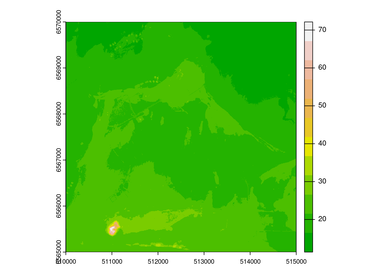

The downloaded data covers a big area while we need a small part of it. Rummu quarry is the small area in the bottom left corner of the figure. Let’s create a bounding box from minimum and maximum x and y coordinates to clip DEM to the area of interest (Rummu Quarry):

#Define the bounding box coordinates
lon <- c(510800, 511300)
lat <- c(6565300, 6565750)

#Create a bounding box using st_bbox
bbox <- data.frame(lon, lat) %>% 
  st_as_sf(coords = c("lon", "lat"), crs = 3301) %>% 
  st_bbox() %>% 
  st_as_sfc()

#Plot the bounding box on top of the DEM
plot(dem, col = terrain.colors(12))
plot(bbox, border = "red", lwd = 2, add = T)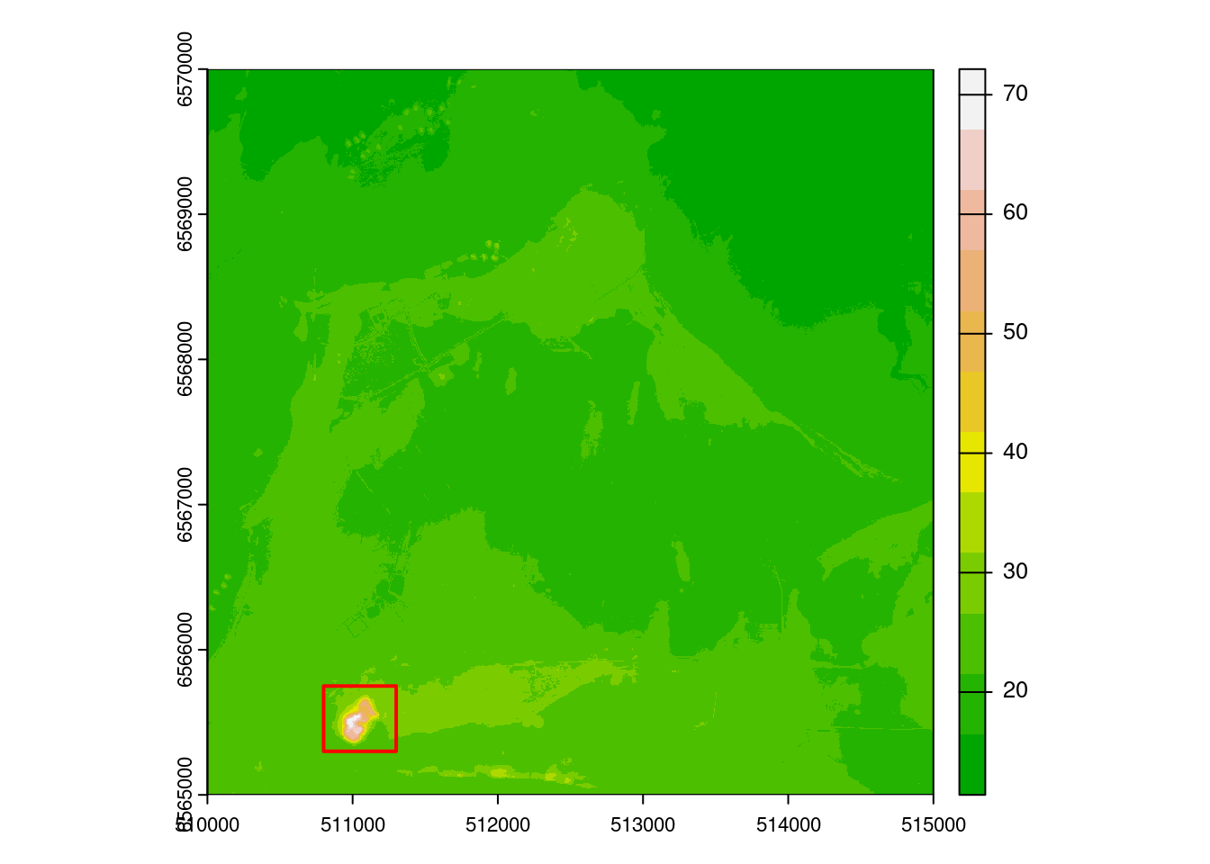

Let’s extract a portion of the DEM based on the bounding box’s extent.

#Crop
dem_crop <- terra::crop(dem, bbox)

#Plot
plot(dem_crop, col = terrain.colors(12))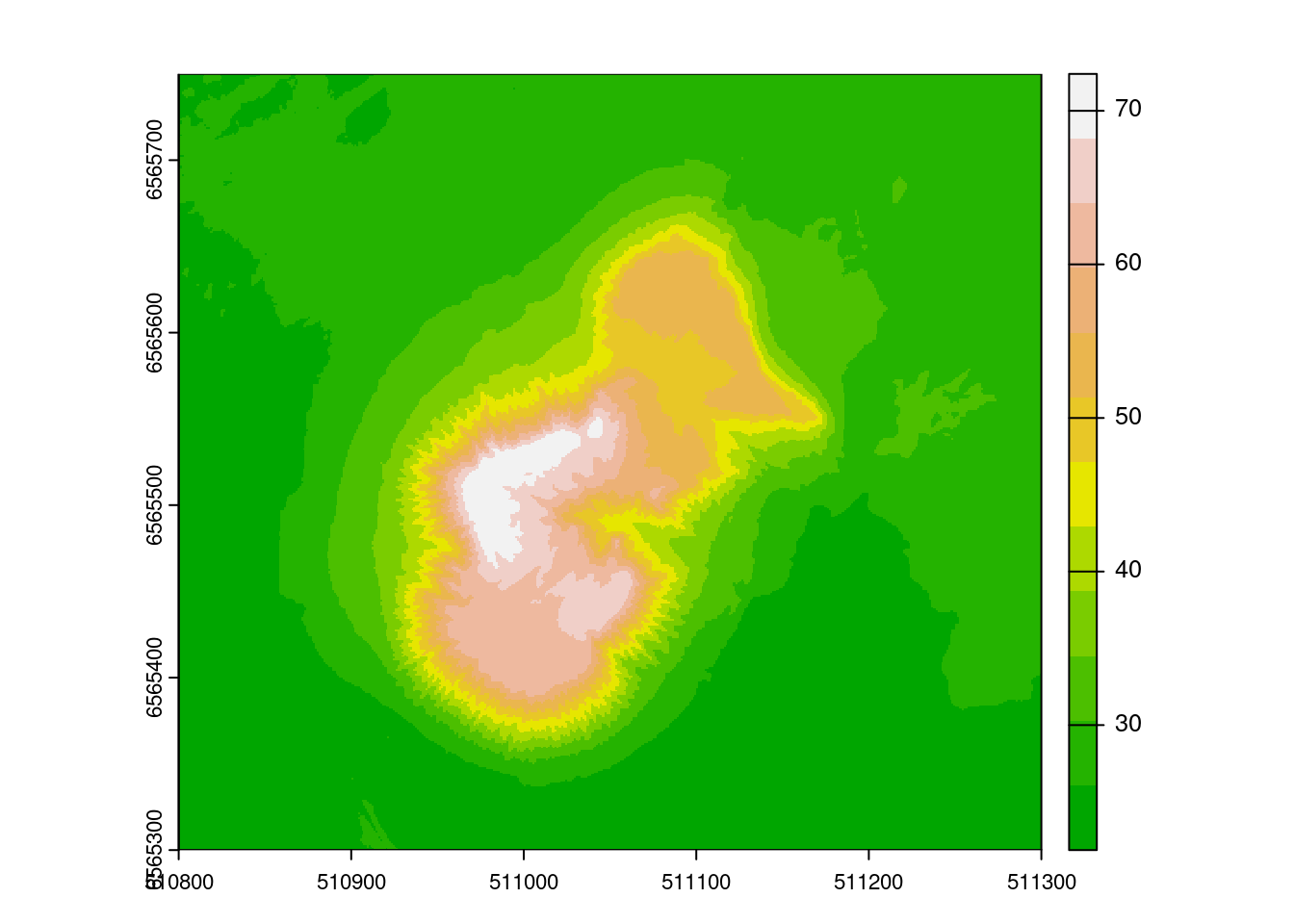

The rayshader package requires elevation data to be in a matrix form for creating 3D terrain maps. So, you need to convert your DEM data from a raster object to a matrix format.

#Convert raster to matrix
dem_matrix <- raster_to_matrix(dem_crop)

Let’s try the first 3D visualization:

dem_matrix %>%
  sphere_shade(texture = "desert") %>%  # applies shading effects to the DEM
  plot_map()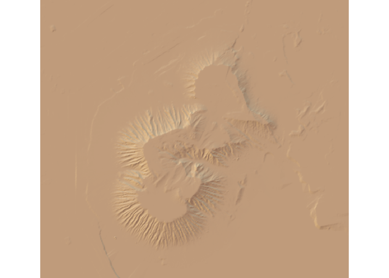

#Try with different textures (`imhof1`,`imhof2`,`imhof3`,`imhof4`,`desert`, `bw`)

We can customize the appearance of a 3D visualization by adjusting some parameters. Here’s an example of how you can change the sunangle and texture parameters. For more information and customization choices, visit this link:

#Adjust sunangle and texture
dem_matrix %>%
  sphere_shade(sunangle = 200, texture = "unicorn") %>% 
  plot_map()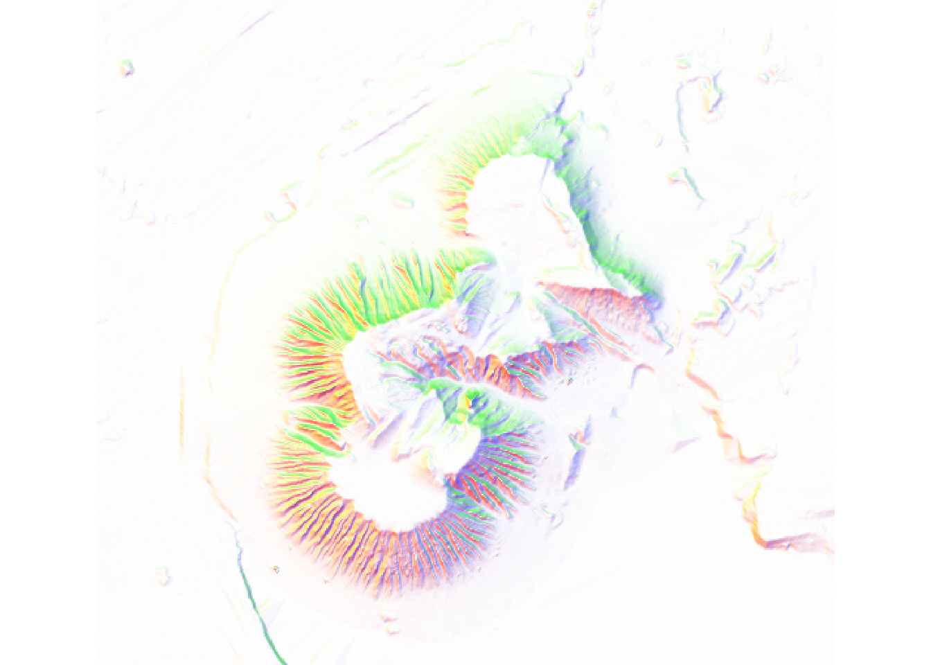

We can also create our own texture and increase the colorintensity (default is 1).

#Apply custom texture and increase color intensity
dem_matrix %>%
  sphere_shade(
    texture = create_texture("#FFA900", "#FF7600", "#A2CDCD", "#CD113B", "#000000"),
    colorintensity = 6) %>% 
  plot_map()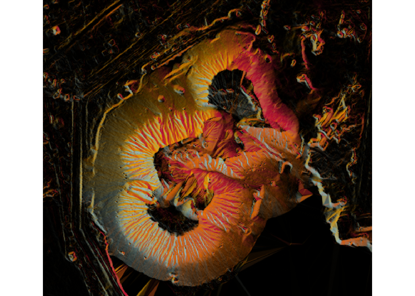

Now, let’s proceed with the 3D visualization using the plot_3d function from rayshader package.

#Use sphere_shade with a custom texture and sun angle
dem_matrix %>%
  sphere_shade(texture = "unicorn", sunangle = 10) %>%
  plot_3d(dem_matrix, 
          baseshape = "hex", # Shape of the base (options: "rectangle", "circle", "hex")
          solidcolor = 'black', # Base color
          solidlinecolor = '#191A19', # Base edge line color
          background = '#1F1D36', # Color of the background
          zscale = 0.4, # Ratio between the x and y spacing
          fov = 0, # Field-of-view angle
          theta = 60, # Rotation around the z-axis
          zoom = 0.7, # Zoom factor
          phi = 45, # Azimuth angle
          windowsize = c(500, 500))  # Size of the plotting window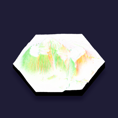

A 3D visualization will appear in a new window, allowing you to customize the perspective of the DEM. Find the optimal viewpoint, and then run the following script. Make sure to keep the newly opened window active during the execution of this code.

Sys.sleep(0.2) # Pause for 0.2 seconds
render_snapshot() # Capture a snapshot of the 3D visualization   

Once we are happy with our shot, we might render it to a high quality image by using the render_highquality() function. When running render_highquality(), there’s no need to pre-compute the shadows with any of the _shade() functions, so we remove those. After rendering, the close3d() function from rgl package is used to close the window displaying the image. Please be patient as it may take a few minutes to complete.

Sys.sleep(0.2)
render_highquality(
  lightdirection = 100,       # Direction of the light source
  lightaltitude = 45,         # Altitude angle of the light source
  lightintensity = 400,       # Intensity of the light source
  clamp_value = 10,           # Clamping value for rendering
  title_text = "Rummu quarry",# Text for the rendering title
  title_color = "white",      # Color of the rendering title text
  title_bar_color = "black",  # Color of the rendering title bar
  parallel = TRUE,            # Flag for parallel rendering
  width = 1000,               # Width of the rendering
  height = 1000,              # Height of the rendering
  samples = 1000)              # Number of rendering samples

# Close the window when you're done
rgl::clear3d()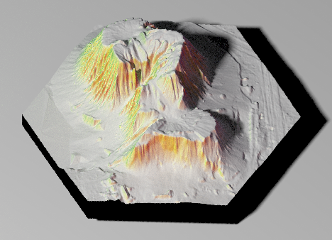

To export high quality resolution images using Rayshader, you need to add a parameter stating the file path and name of the output image in render_snapshot().

#Export a map
render_snapshot("Rummu.png", clear = TRUE)

The Rummu heap is located nearby the water body. We can represent this water feature, assuming that any terrain below 23 meters in elevation is submerged or flooded.

dem_matrix %>%
  sphere_shade(texture = "imhof1", sunangle = 100) %>%
  plot_3d(
    dem_matrix,
    baseshape = "circle",     # Shape of the base
    solidcolor = 'grey20',    # Base color
    solidlinecolor = 'grey20',# Base edge line color
    zscale = 0.4,             # Ratio between x and y spacing
    fov = 0,                  # Field-of-view angle
    theta = 60,               # Rotation around the z-axis
    zoom = 0.7,               # Zoom factor
    phi = 45,                 # Azimuth angle
    windowsize = c(500, 500), # Window size
    water = TRUE,             # Display water surface
    waterdepth = 23,          # Elevation below which terrain is considered flooded
    wateralpha = 0.5,         # Transparency of the water surface
    watercolor = "#233aa1",   # Color of the water
    waterlinecolor = "white", # Color of the waterline
    waterlinealpha = 0.5)      # Transparency of the waterline
  
Sys.sleep(0.2)        
render_snapshot()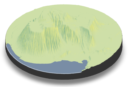     

To enhance our 3D visualization and its information content, let’s incorporate details from a 20-cm aerial image. Download the aerial image from Landboard Estonia using this link. Ensure that you select the image corresponding to the same sheet number that you used for downloading the DEM (63613) and select 63613_OF_RGB_GeoTIFF_2022_06_15.zip.

Import the downloaded aerial image and crop the image to the extent of previously created bbox object.

#Import aerial image
rgb <- rast("63613_RGB.tif")

#Crop
rgb_cropped <- terra::crop(rgb, bbox)

#Plot the RGB image
plotRGB(rgb_cropped)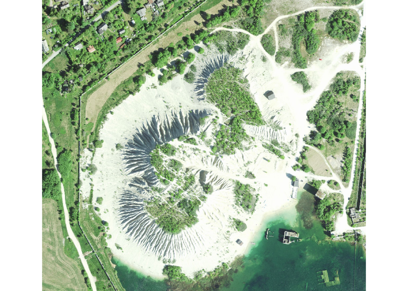

Similar to what we did for the DEM data, we also need to transform the RGB image into a matrix. It’s important to note that each band (Red, Green, Blue) should be converted individually.

#Assign names to the bands in the cropped image
names(rgb_cropped) <- c("r", "g", "b")

#Convert each band (Red, Green, Blue) to a matrix
image_R <- rayshader::raster_to_matrix(rgb_cropped$r) # Red band
image_G <- rayshader::raster_to_matrix(rgb_cropped$g) # Green band
image_B <- rayshader::raster_to_matrix(rgb_cropped$b) # Blue band

#Create an RGB array and assign the color channels
image_RGB <- array(0, dim = c(nrow(image_R), ncol(image_R), 3))
image_RGB[,,1] <- image_R # assign the values of the image_R matrix to the red channel
image_RGB[,,2] <- image_G # assign the values of the image_G matrix to the green channel
image_RGB[,,3] <- image_B # assign the values of the image_B matrix to the blue channel

#Rescale the image to the [0, 1] range
image_RGB <- scales::rescale(image_RGB, to = c(0, 1))

#Plot 
plot_map(image_RGB)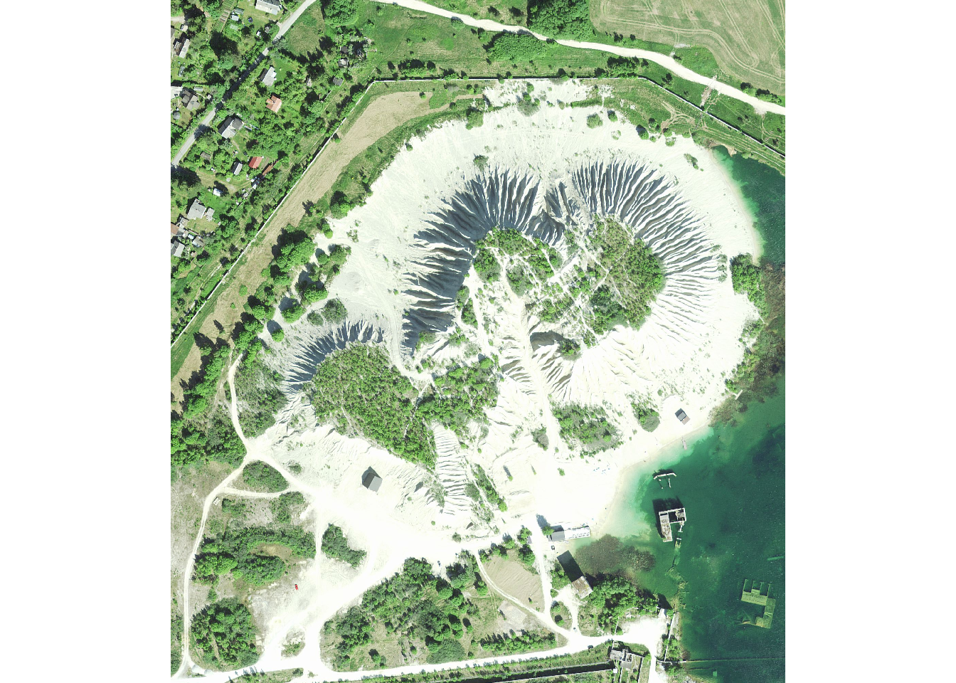

Next up, let’s add the RGB image onto the DEM. Ensure that the subsequent processes depend on the persistence of the newly opened window initiated by the next code.

plot_3d(
  image_RGB,         # RGB image to be plotted
  dem_matrix,        # DEM matrix
  windowsize = c(700, 600),   # Size of the plotting window in pixels
  zscale = 0.6,      # Ratio between the x and y spacing
  shadowdepth = -50, # Depth of shadows
  zoom = 0.7,        # Zoom factor
  phi = 45,          # Azimuth angle
  theta = -45,       # Rotation around the z-axis
  fov = 70,          # Field-of-view angle
  background = "#D5D5D5",  # Background color
  shadowcolor = "#5e5e5e")  # Color of shadows

Sys.sleep(0.2) 
render_snapshot()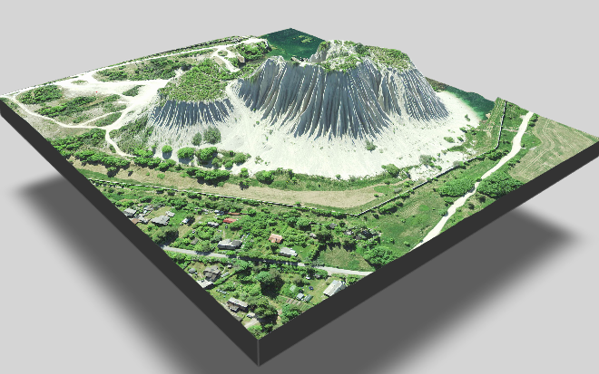

You can add labels to the plot (find more information on how to do this here. For example, add one viewing point and diving place:

# Add a label for the viewing point
render_label(
  dem_matrix,       # Demographic matrix or data
  x = 180,          # X-coordinate for label placement
  y = 240,          # Y-coordinate for label placement
  altitude = 30,    # Altitude of the label in 3D space
  zscale = 0.6,     # Scaling factor for the label in the z-direction
  text = "Viewing point", # Text content of the label
  textcolor = "black", # Color of the label text
  linecolor = "black", # Color of the label outline
  dashed = TRUE,       # Flag indicating whether the label should have a dashed outline
  alpha = 0.9,         # Transparency level of the label
  textsize = 1.5)       # Size of the label text

# Add a label for the diving place
render_label(
  dem_matrix,       
  x = 390,          
  y = 370,          
  altitude = 60,    
  zscale = 0.6,     
  text = "Diving place",   
  textcolor = "black",    
  linecolor = "black",    
  dashed = TRUE,           
  alpha = 0.9,             
  textsize = 1.5)

# Capture a snapshot of the visualization with a title
render_snapshot(
  title_text = "Rummu quarry \nData: Land Board",  # Text for the snapshot title
  title_color = "white",  # Color of the snapshot title text
  title_bar_alpha = 1) # Transparency level of the title bar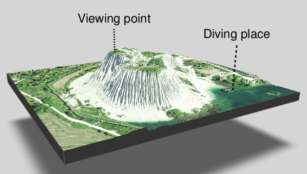

8.3. 3D animation with rayshader

The fundamental capability of the rayshader package lies in its ability to generate 3D animations. To produce animations, we can employ the render_snapshot function to save individual frames. These frames can then be assembled into a cohesive animation using the av_encode_video function, which is part of the av package.

Following the selection of an aesthetically pleasing viewpoint for the above visualization, the subsequent two code chunks can be executed to generate a video centered around the heap. The first chunk generates 360 images, each representing a degree of view (for a total of 360 degrees), and the second chunk compiles these images into a video.

#Let's create a new folder to store the images:
dir.create("./image")

# Generate a sequence of angles from 0 to 360 with one image for each degree
angles <- seq(0,360, length.out = 361)[-1] 

# Loop through each angle to render and save the images
for(i in 1:360) {
  # Adjust the camera angle based on the current iteration
  render_camera(theta = -45 + angles[i])
  # Render the scene and save the snapshot image
  render_snapshot(filename = sprintf("./image/Rummu_quarry%i.png", i), 
                  title_text = "./image/Rummu quarry \nData: Land Board",
                  title_color = "white", 
                  title_bar_alpha = 1)}

rgl::clear3d()

Let’s create a video with those 360 images:

# Generate a vector of file paths for a series of images (in PNG format)
av::av_encode_video(
  sprintf("./image/Rummu_quarry%d.png",seq(1,360, by = 1)), 
  framerate = 30, # frame rate for the video (30 frames per second)
  output = "./image/Rummu_quarry.mp4") # Specify the output path and name

8.4. 3D mapping with rayshader and ggplot2

One of the pretty features of the Rayshader package is its ability to transform ggplot2 objects to visually 3D. The plot_gg() function from Rayshader package facilitates the transformation of ggplot objects into a 3D format, projecting the fill or color aesthetic onto a third dimension. To demonstrate the creation of 3D visualizations using ggplot2, we will employ population data introduced in lesson 1.

In the next few lines of code, we use the ggplot() function from the ggplot2 package to produce the gg_map. The geom_sf() function loads the polygon data from the Population field, and we also define the color coding through scale_fill_viridis() function that accepts a column (Population) to define the color coding. Then, the final lines of code use the plot_gg() function from the rayshader package to display the data in 3D. Notice map produced by the ggplot() function is passed to the plot_gg() function.

#Import population data from lesson 1 folder
est_pop <- st_read("../R_01/population.gpkg") 

#Create ggplot 
gg_map <- ggplot(data = est_pop) +
  geom_sf(aes(fill = Population)) +
  scale_fill_viridis() +
  ggtitle('Population Distribution in Estonia') +
  theme_dark()

#Plot in 3D using the plot_gg function
plot_gg(
  gg_map,           # Input ggplot object to be rendered in 3D
  multicore = TRUE, # Flag to use multiple processor cores for faster rendering
  width = 5,        # Set the width of the resulting 3D plot
  height = 5,       # Set the height of the resulting 3D plot
  scale = 250,      # Vertical exaggeration of the 3D plot
  zoom = 0.55,      # Zoom level of the plot
  theta = 45,       # Azimuth angle (angle of the light source around the x-axis)
  phi = 30,         # Altitude angle (angle of the light source above the x-y plane)
  sunangle = 225,   # Angle of the light source for shading
  windowsize = c(1400,866)) # Size of the plotting window in pixels
  
Sys.sleep(0.2)
render_snapshot()

Upon completing the 3D visualization for the ggplot object, the rendered result can be saved using the render_movie function. It is crucial to ensure that the new window generated through the preceding code remains open when executing this section of code.

# Set the output file path and name for the rendered movie
outputFile <- file.path("estonia_population.mp4")

# Call the render_movie function to generate the movie
render_movie(filename = outputFile)

The created video can be visualized using the embed_video() function from the embedr package.