library(tidyverse)    # For data manipulation and plotting
library(sf)           # For handling geographic data using simple features
library(magick)       # For manipulating and processing image files
library(terra)        # For analyzing raster data and working with spatial datasets
library(tmap)         # For creating thematic maps to visualize spatial patterns
library(spData) # For accessing various spatial datasets for practiceLesson 10: Animations
This lesson focuses the creation of animated maps or plots in R, offering a dynamic and engaging approach to interact with data and visualize it over time or through a sequence of events. The codes and materials utilized in this lesson have been adapted from the original materials created by Anto Aasa.
At the end of this lesson, the students should be able to:
- Understand how to animate spatial data in R
- Explore and visualize temporal patterns in data using R animations
- Customize animation parameters based on specific data characteristics
This lesson requires the following packages:
10.1. Introduction
Creating animations ((rapid succession of sequential images)) is an incredibly valuable technique for presenting information in an engaging and interactive ways. Animated maps can be very helpful in illustrating concepts or discovering relationships, which makes them very helpful in teaching and exploratory research. The animation of spatial data entails displaying a sequence of images swiftly, enabling a smooth transition between different data states. A compelling visualization not only captures the audience’s interest but also leaves a lasting impression.
In general animations can be created for two purposes:
- process animation (changes in time),
- animation of static plot to reveal different angles.
Creating animated graphs in R is fairly straightforward, once you have the right tools and understand a few basic principles about how the animations are created. In this lesson, we will go through the essential steps needed to create simple yet impactful animations using the Estonian border and DEM datasets introduced in the preceding lessons.
10.2. Animations of image sequences
Creating animations from a sequence of images involves combining multiple images into a continuous visual presentation, giving the illusion of motion or change over time. In this example, we’ll generate an animation showing the transformation of Estonia’s border outline as it undergoes a simplification process. To commence, let’s import the data representing the borders of Estonia (estonian_border.gpkg), which was introduced in lesson 4.
# Import data
estonia <- st_read("../R_04/estonian_border.gpkg")
Reading layer `eestimaa' from data source
`/home/geoadmin/dev/simply-general/teaching/geospatial_python_and_r/R_04/estonian_border.gpkg'
using driver `GPKG'
Simple feature collection with 1 feature and 2 fields
Geometry type: MULTIPOLYGON
Dimension: XY
Bounding box: xmin: 21.77134 ymin: 57.50842 xmax: 28.21073 ymax: 59.68583
Geodetic CRS: WGS 84# Transform it to EPSG 3301
est_bor <- st_transform(estonia, 3301)Now, we’ll generate a sequence of images, where each subsequent image is slightly more simplified than the previous one. Initially, we’ll create a vector specifying the simplification level (dTolerance) for each step:
# Create data frame, where first value of dTolerance is 102
steps <- data.frame(step = 102) # 102 comes after testing different values

# Run the for loop to create the vector:
for(j in 1 : 100){
  steps_tmp <- steps[j,]  # Extract the j-th row from 'steps' data frame
  steps_tmp <- 1.07 * steps_tmp # Multiply each element in the row by 1.07
  steps <- rbind(steps, data.frame(step = steps_tmp)) # Create a new data frame with the modified row
}
Let’s check the output:
# First 10 steps:
head(steps, n = 10)
step
1 102.0000
2 109.1400
3 116.7798
4 124.9544
5 133.7012
6 143.0603
7 153.0745
8 163.7897
9 175.2550
10 187.5228Next, we’ll establish a stable frame around Estonia to avoid any erratic movement in the animation. This will be achieved by utilizing a bounding box, which will undergo a transformation into a polygon:
# Calculate the bounding box of est_bor
bbox <- st_bbox(est_bor)

# Convert the bounding box to a dataframe
bbox_df <- data.frame(x = c(bbox[1], bbox[3]), y = c(bbox[2], bbox[4]))

# Create an sf object with the bounding box
bbox_sf <- st_as_sf(bbox_df, coords = c("x", "y"), crs = 3301)
Let’s visualize both the bounding box and the Estonia contour on the same plot:
tmap_mode("plot") tmap mode set to plottingtm_shape(bbox_sf)+
tm_dots("red", size= 2, shape = 3) +
tm_shape(est_bor)+
tm_borders()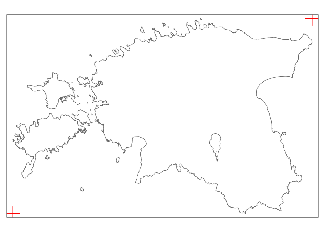
To keep the stuff tidy, we create sub-directory (called cont_anim) for animation frames. Let’s move on to generating animation frames using a straightforward for loop, where a simplified contour is produced for each step of simplification.
# Create a folder to save individual frames
dir.create("cont_anim")
Warning in dir.create("cont_anim"): 'cont_anim' already exists# Create the image for every generalization step
for(i in 1 : nrow(steps)){
est_bor_ee <- est_bor # create copy of border
est_bor_ee <- st_simplify(est_bor_ee, dTolerance = steps[i,1])
# Generate a frame name with left-padded zeros
frameName <- str_pad(i, 4, side = "left", pad = "0")
# Create a ggplot object
myplot <- ggplot()+
theme_minimal()+
geom_sf(data = bbox_sf, colour="white")+
geom_sf(data = est_bor_ee)
# Save the frame as a PNG file
ggsave(filename = paste0("cont_anim/frame_", frameName, ".png"),
plot = myplot, dpi = 100, width = 5, height = 4, units = "in")
}You should now have 101 images depicting the border of Estonia, all stored within cont_anim sub-folder. Next, we will compile a directory listing of these file names, concatenate them to create an animated GIF, and save the resultant animation utilizing the magick package. The processing will take a few minutes:
# List file names in the 'cont_anim' folder and read them into a list
cont_files <- list.files("cont_anim", pattern = ".png", full.names = TRUE)
cont_list <- lapply(cont_files, image_read)

# Join the images together
cont_join <- image_join(cont_list)

# Animate the joined images at 10 frames per second
cont_anim <- image_animate(cont_join, fps = 10)

# Save the animated image as a GIF
image_write(cont_anim, path = "cont_anim.gif")
Warning in image_write(cont_anim, path = "cont_anim.gif"): Writing image with 0
framesThe resulting image should be something like this:
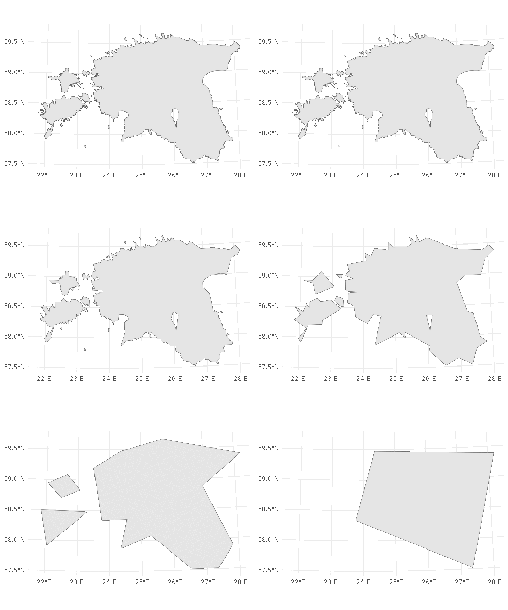
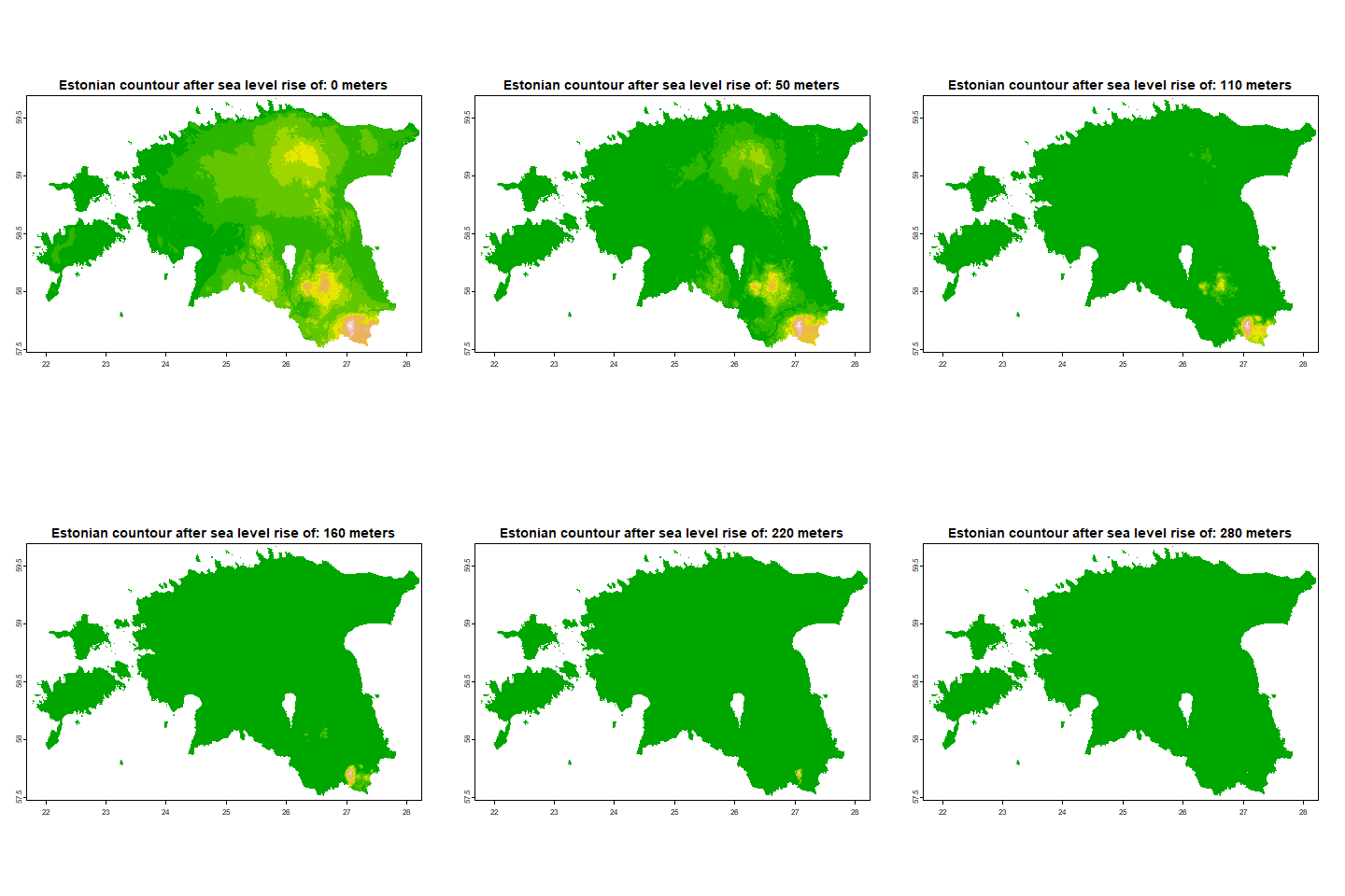
Let’s consider another example demonstrating the animation of image sequences using changes in the Estonian contour due to rising sea levels. While the example is simplistic and not representative of actual scenarios, it serves as an effective learning example. To undertake this task, we’ll utilize the elevation layer of Estonia, which can be imported from lesson 5.
# Load the DEM from lesson 5
dem <- rast("../R_05/dem_est.tif")

# Project the DEM to a new CRS (e.g., EPSG:3301) using bilinear interpolation with a resolution of 100 units
dem_proj <- project(dem, "+init=epsg:3301", method = "bilinear", res = 100)
Warning in x@cpp$warp(SpatRaster$new(), y, method, mask, FALSE, FALSE, opt):
GDAL Message 1: +init=epsg:XXXX syntax is deprecated. It might return a CRS
with a non-EPSG compliant axis order.Next, we create animation steps. It means we create the sequence of height above sea level in meters (from -10 to 280 meters)
# Create a folder to save individual frames
dir.create("elev_anim")

# Define a sequence of sea level rise values
elev_range <- seq(-10, 280, by = 10)

#Loop through each sea level rise scenario and create frames
for (sea_level_rise in elev_range) {
  dem_copy <- dem  # Create a copy of the original DEM
  dem_copy <- clamp(dem_copy, sea_level_rise, Inf)

  # Save the frame as PNG
  png(filename = paste0("elev_anim/frame_", sea_level_rise, ".png"))
  plot(dem_copy, col = terrain.colors(10),
       main = paste("Estonian countour after sea level rise of:",
                    sea_level_rise, "meters"), legend = FALSE)
  # Close the PNG device
  dev.off()
}

# List all PNG files in the folder in ascending order
elev_files <- list.files("elev_anim", pattern = ".png", full.names = TRUE)

# Order the file names based on numeric values extracted from the file names
elev_files <- elev_files[order(as.numeric(gsub("[^0-9]", "", elev_files)))]

# Read each PNG file into a list of magick images
elev_list <- lapply(elev_files, image_read)

# Combine the images into a single animation frame
elev_join <- image_join(elev_list)

# Create an animated GIF
elev_anim <- image_animate(elev_join, fps = 5)

# Write the animated GIF to the specified path
image_write(elev_anim, path = "elev_anim.gif")
The result should be something like this:
Let’s assume that we possess the data indicating the presence of an unknown flying object circling over Estonia. Our goal is to create an animation indicating this flying object utilizing the Estonian border dataset. This example is again very abstract but will help to better understand the process of animating image sequences.
Let’s begin by calculating the centroid of Estonia and establishing a 100 km buffer around it:
# Calculate centroids of polygons
est_cntr_sf <- st_centroid(est_bor)

# Create buffer zones around centroids
est_cntr_buf <- st_buffer(est_cntr_sf, dist = 100000)
Plot it:
# Create a thematic map with borders from 'est_bor'
tm_shape(est_bor) +
  tm_borders() +

# Add borders from 'est_cntr_buf' in red with a line width of 2
tm_shape(est_cntr_buf) +
  tm_borders("red", lwd = 2)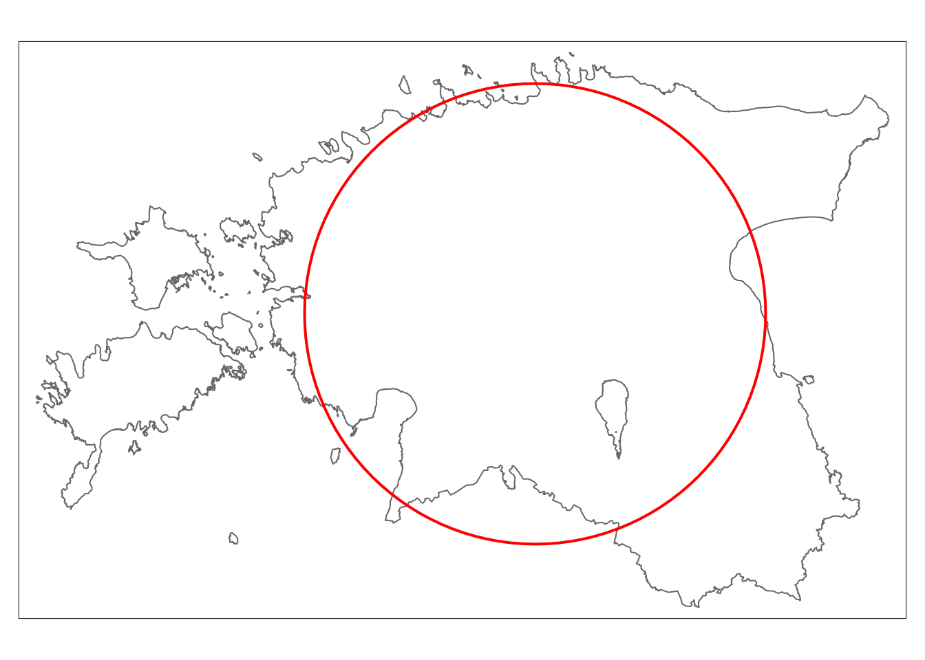
The circle is a polygon defined by points which are connected with each other. Convert the polygon to points:
# Get coordinates as data frame
est_cntr_buf_df <- st_coordinates(est_cntr_buf) %>%
  as_tibble()

# Rank the coordinates
est_cntr_buf_df <- est_cntr_buf_df %>%
  mutate(rnk = seq(1, nrow(est_cntr_buf_df), 1))

# Plot it
ggplot()+
  theme_minimal()+
  geom_sf(data= est_bor, col = "grey", fill = "grey97", size = 0.25)+
  geom_point(data = est_cntr_buf_df, aes(x = X, y = Y, size= rnk, alpha= rnk), col = "red")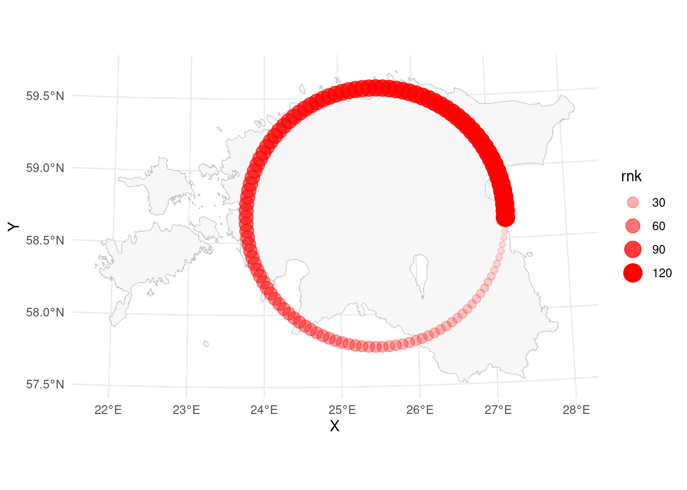
As you notice we are using alpha to add the fading tail to our moving dots. Currently it’s too long. We should add it to 10 location points. Now our task is to create animation frames. But firstly we should design the single animation frame:
# First 10 points
est_cntr_buf_df_tmp <- est_cntr_buf_df[1:10,]

# Plot
ggplot()+
  theme_minimal() +
  geom_sf(data = est_bor, col = "grey", fill = "grey97", size = 0.25) +
  geom_path(data = est_cntr_buf_df, aes(x = X, y = Y), col = "pink", size = 0.1) +
  geom_point(data = est_cntr_buf_df_tmp,
             aes(x= X, y = Y, alpha = rnk, size = rnk), colour = "red") +
  scale_alpha(range = c(0, 1)) +
  scale_size(range = c(0.5, 4))
Warning: Using `size` aesthetic for lines was deprecated in ggplot2 3.4.0.
ℹ Please use `linewidth` instead.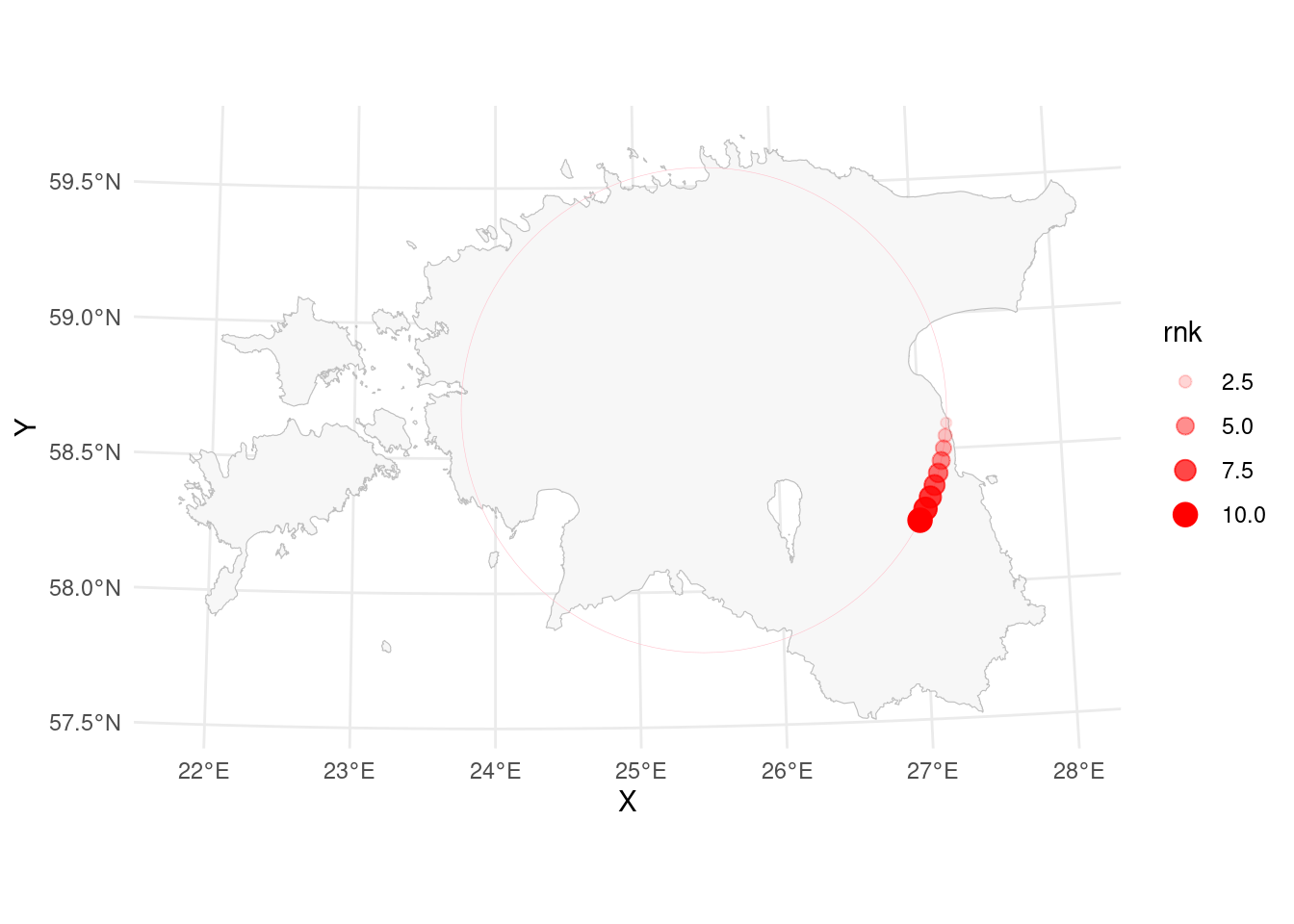
Our dataset contains 121 location points. This means we can create single animation frame for every dot. But firstly we have to create again the numbering of images:
#Calculate the number of characters in rank (new column):
est_cntr_buf_df <- est_cntr_buf_df %>%
  mutate(rnk_nchar = nchar(rnk))

#Create separate data frame for image name prefixes:
rnk_joiner <- data.frame(rnk_nchar = c(1, 2, 3),
                         prefix = c("00", "0", NA))
#Join two table:
est_cntr_buf_df <- left_join(est_cntr_buf_df, rnk_joiner)
Joining with `by = join_by(rnk_nchar)`#Calculate the rank as character
est_cntr_buf_df <- est_cntr_buf_df %>%
mutate(frame_name = ifelse(!is.na(prefix), paste0(prefix, rnk), rnk))Create animation frames and save them as png-files.
# Create sub-directory for animation frames
dir.create("fly_anim", showWarnings = FALSE)

# Iterate through each frame
for (i in 1:nrow(est_cntr_buf_df)) {
  # Subset data for the current frame
  est_cntr_buf_df_tmp2 <- est_cntr_buf_df %>%
    filter(rnk > i - 1 & rnk < i + 10)

  # Extract data for the head point in the current frame
  est_cntr_buf_df_head <- est_cntr_buf_df %>%
    filter(rnk == i + 10)

  # Create a ggplot for the current frame
  ggplot() +
    theme_light() +
    geom_sf(data = est_bor, col = "grey", fill = "grey97", size = 0.25) +
    geom_path(data = est_cntr_buf_df, aes(x = X, y = Y), col = "pink", size = 0.1) +
    geom_point(data = est_cntr_buf_df_tmp2, aes(x = X, y = Y, alpha = rnk, size = rnk), colour = "orange") +
    geom_point(data = est_cntr_buf_df_head, aes(x = X, y = Y), colour = "darkred", size = 2.5) +
    scale_alpha(range = c(0, 0.7)) +
    scale_size(range = c(0.2, 2)) +
    guides(alpha = FALSE, size = FALSE)

  # Generate the frame name with zero-padding
  frame_name <- sprintf("fly_anim/frame_%04d.png", i)

  # Save the plot as a PNG file
  ggsave(filename = frame_name, dpi = 200, height = 3, width = 4.5)
}
For animation bind the images together using magick package:
# List image files
fly_files <- list.files("fly_anim", pattern = ".png", full.names = TRUE)

# Read images
fly_list <- lapply(fly_files, image_read)

# Append images to create an animated GIF
fly_join <- image_join(fly_list)

# Create an animated GIF
fly_anim <- image_animate(fly_join, fps = 25)

# Write the animated GIF to the specified path
image_write(fly_anim, path = "fly_anim.gif")
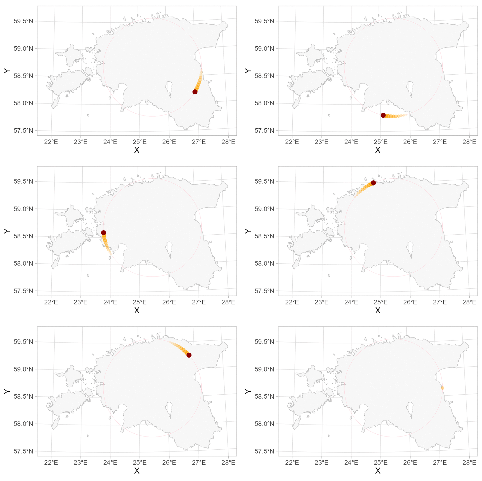
The resulting gif image should be something like this:
10.3. Animations of changes in time
Animation for time series data aids in visualizing the evolution of data over a time. It involves generating a sequence of frames or images that depict how data points change and develop as time progresses.
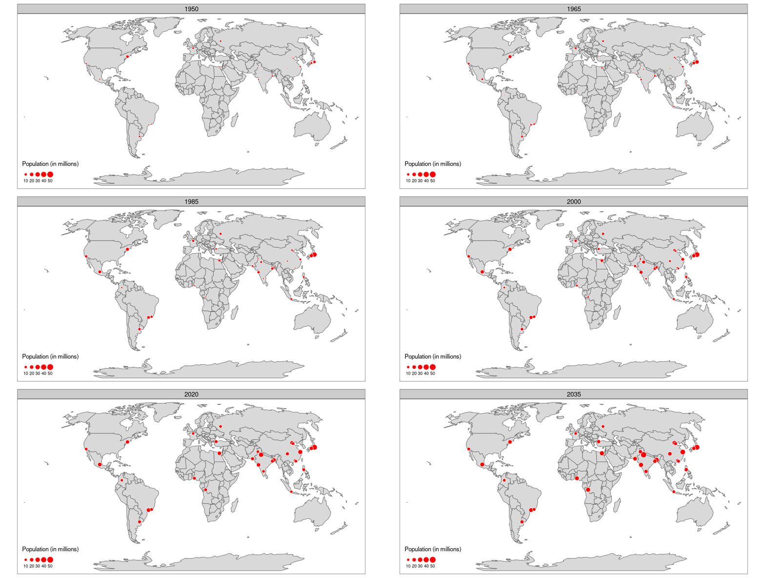
To illustrate the concept of time series animation, let’s make use of the urban_agglomerations dataset from the spData package. The faceted plots we created in lesson 4, can show how spatial distributions of variables change (e.g., over time). However, they become tiny for large data, and yield physically separated on the screen or page means that subtle differences between facets can be hard to detect. Animated maps eliminate the problem of overcrowding multiple maps on a single screen, allowing viewers to observe the dynamic evolution of the spatial distribution of the world’s most populous agglomerations over time.
Let’s first load the dataset and perform some data preparation tasks.
# Load data from spData package
urb_agg <- spData::urban_agglomerations  # Urban agglomerations data
world_polygons <- spData::world  # World map polygons data

# Transform the world map to a World Robinson projection
world.robin <- st_transform(world_polygons, "+proj=robin +lon_0=0 +x_0=0 +y_0=0 +ellps=WGS84 +datum=WGS84 +units=m +no_defs")
Then, create an animation:
# Create a thematic map for urban aggregation using tmap
urb_anim <- tm_shape(world.robin) +
  tm_polygons() +  # Add base map polygons
  tm_shape(urb_agg) +  # Overlay urban aggregation data
  tm_symbols(
    size = "population_millions",  # Symbol size based on population_millions variable
    col = "red",  # Symbol color
    title.size = "Population (in millions)",  # Legend title for symbol size
    border.col = "white") + # Symbol border color
  tm_facets(
    by = "year",  # Facet by the 'year' variable
    nrow = 1,  # Arrange facets in one row
    ncol = 1,  # Arrange facets in one column
    free.coords = FALSE)  # Ensure consistent coordinates across facets

# Combine separate maps for each year into an animated GIF
tmap_animation(urb_anim, filename = "urb_agglo_anim.gif", delay = 30)
The animated map should look like this:
