import matplotlib.pyplot as plt
import matplotlib as mpl

import osmnx as ox

place_name = "Tartu, Estonia"
graph = ox.graph_from_place(place_name)
type(graph)networkx.classes.multidigraph.MultiDiGraph![]()
OpenStreetMap (OSM) is a global collaborative (crowd-sourced) dataset and project that aims at creating a free editable map of the world containing a lot of information about our environment. It contains data for example about streets, buildings, different services, and landuse to mention a few.
OSM has a large userbase with more than 4 million users that contribute actively on OSM by updating the OSM database with 3 million changesets per day. In total OSM contains more than 4 billion nodes that form the basis of the digitally mapped world that OSM provides (stats from November 2017.
OpenStreetMap is used not only for integrating the OSM maps as background maps to visualizations or online maps, but also for many other purposes such as routing, geocoding, education, and research. OSM is also widely used for humanitarian response e.g. in crisis areas (e.g. after natural disasters) and for fostering economic development (see more from Humanitarian OpenStreetMap Team (HOTOSM) website.
This lesson we will explore a new and exciting Python module called osmnx that can be used to retrieve, construct, analyze, and visualize street networks from OpenStreetMap. In short it offers really handy functions to download data from OpenStreet map, analyze the properties of the OSM street networks, and conduct network routing based on walking, cycling or driving.
There is also a scientific article available describing the package:
- Boeing, G. 2017. "OSMnx: New Methods for Acquiring, Constructing, Analyzing, and Visualizing Complex Street Networks." Computers, Environment and Urban Systems 65, 126-139. doi:10.1016/j.compenvurbsys.2017.05.004
As said, one the most useful features that osmnx provides is an easy-to-use way of retrieving OpenStreetMap data (using OverPass API ).
Let's see how we can download and visualize street network data from a district of Tartu in City Centre, Estonia. Osmnx makes it really easy to do that as it allows you to specify an address to retrieve the OpenStreetMap data around that area. In fact, osmnx uses the same Nominatim Geocoding API to achieve this which we tested during the Lesson 2.
Let's retrieve OpenStreetMap (OSM) data by specifying "Tartu, Estonia" as the address where the data should be downloaded.
import matplotlib.pyplot as plt
import matplotlib as mpl
import osmnx as ox
place_name = "Tartu, Estonia"
graph = ox.graph_from_place(place_name)
type(graph)networkx.classes.multidigraph.MultiDiGraphOkey, as we can see the data that we retrieved is a special data object called networkx.classes.multidigraph.MultiDiGraph. A DiGraph is a data type that stores nodes and edges with optional data, or attributes. What we can see here is that this data type belongs to a Python module called networkx that can be used to create, manipulate, and study the structure, dynamics, and functions of complex networks. Networkx module contains algorithms that can be used for example to calculate shortest paths along networks using e.g. Dijkstra's or A* algorithm.
Let's see how our street network looks like. It is easy to visualize the graph with osmnx with plot_graph() function. The function utilizes Matplotlib for visualizing the data, hence as a result it returns a matplotlib figure and axis objects.
ox.plot_graph(graph)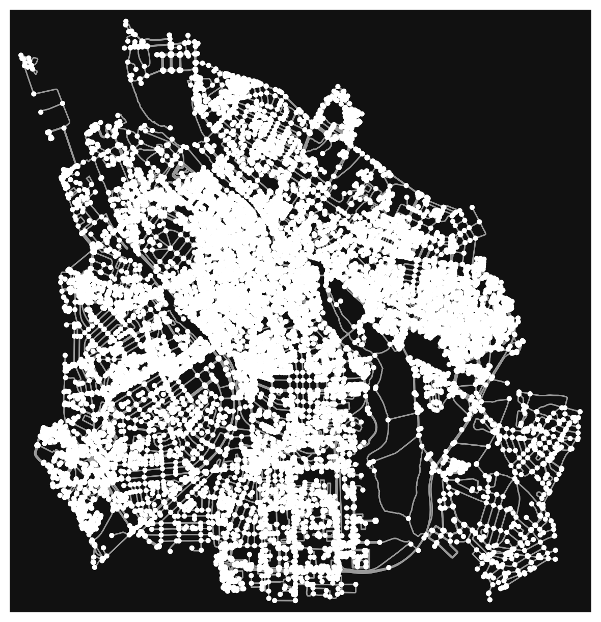
Great! Now we can see that our graph contains the nodes (circles) and the edges (lines) that connects those nodes to each other.
Let's explore the street network a bit. The library allows us to convert the nodes and edges dataset into two separate geodataframes.
nodes, edges = ox.graph_to_gdfs(graph)
print(edges.head(3))
print(edges.crs)
osmid highway service oneway reversed \
u v key
8220881 1250012238 0 1244506595 service driveway False False
11568460574 0 29394188 trunk NaN True False
8220933 6854135436 0 117178126 trunk NaN True False
length lanes maxspeed name ref \
u v key
8220881 1250012238 0 10.069150 NaN NaN NaN NaN
11568460574 0 51.365064 2 50 Riia 3
8220933 6854135436 0 47.330961 5 50 Riia 3
geometry \
u v key
8220881 1250012238 0 LINESTRING (26.71898 58.37259, 26.71887 58.37266)
11568460574 0 LINESTRING (26.71898 58.37259, 26.71893 58.372...
8220933 6854135436 0 LINESTRING (26.73016 58.37857, 26.72998 58.378...
bridge junction width access tunnel
u v key
8220881 1250012238 0 NaN NaN NaN NaN NaN
11568460574 0 NaN NaN NaN NaN NaN
8220933 6854135436 0 NaN NaN NaN NaN NaN
epsg:4326As you will see, there are several interesting columns, for example:
But like with all data we get from somewhere else, we need to check datatypes and potentially clean up the data. Let's look at the speed limit maxspeed information that is entered in the OSM dataset for many streets. Here is again a very manual and defensive way of making sure to convert the information in the maxspeed column into a predictable numerical format.
def clean_speed(x):
    try:
        if isinstance(x, str):
            return float(x)
        elif isinstance(x, float):
            return x
        elif isinstance(x, int):
            return x
        elif isinstance(x, list):
            return clean_speed(x[0])
        elif x is None:
            return 20
        elif np.isnan(x):
            return 20
        else:
            return x
    except:
        print(type(x))
        return 20

edges['speed'] = edges['maxspeed'].apply(clean_speed)
Now let's have a more colourful look at the streets of Tartu, based on the estimated max-speed attribute. Let's also reproject to Estonian National Grid (EPSG:3301):
streets_3301 = edges.to_crs(3301)

fig, ax = plt.subplots(figsize=(10,8))

streets_3301.plot(ax=ax, column='speed', cmap='viridis', legend=True)
plt.title("OSM coded max-speed of streets in Tartu")
plt.show()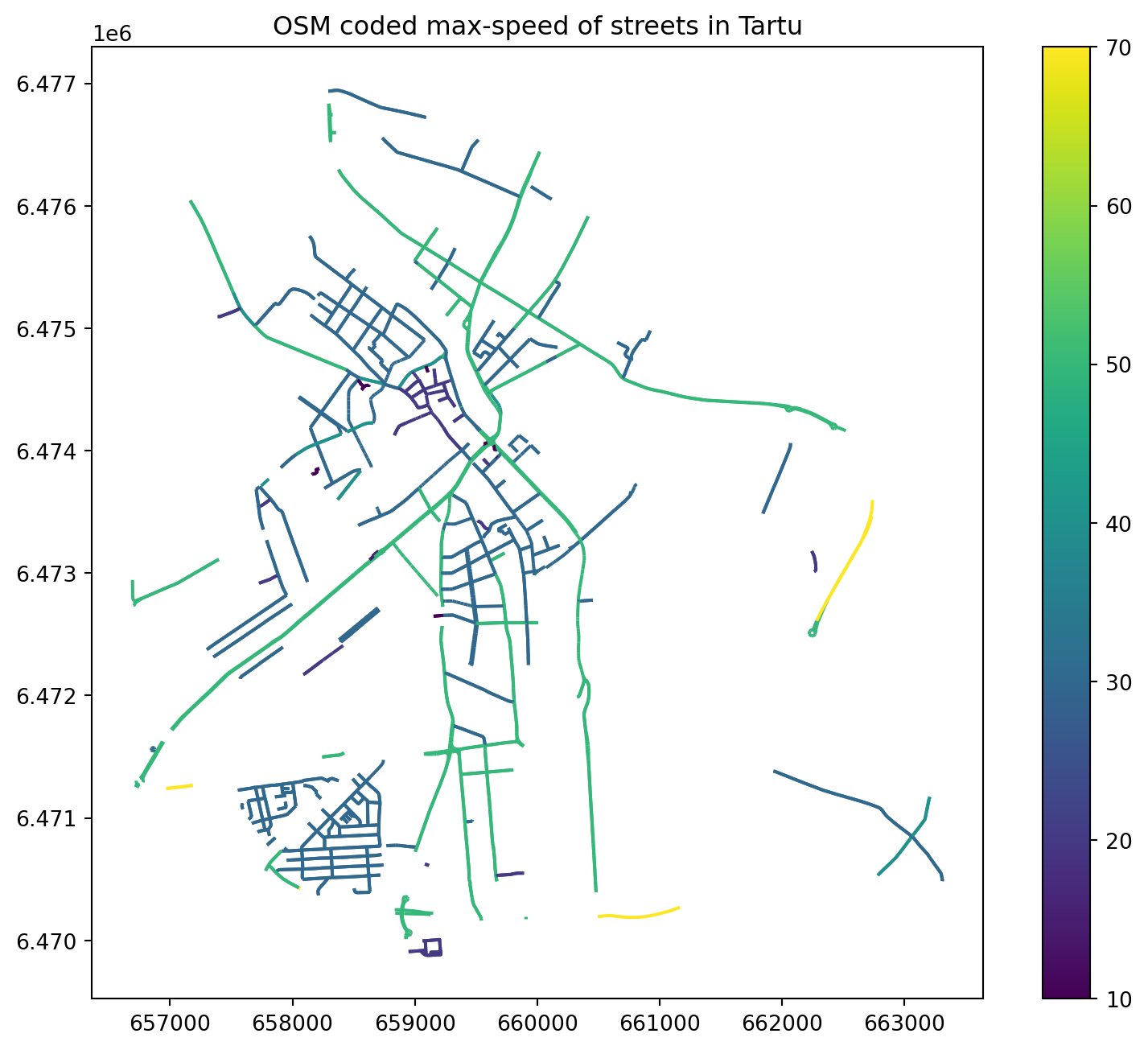
It is also possible to retrieve other types of OSM data features with osmnx.
Let's download the buildings with features_from_place() function and plot them on top of our street network in Tartu.
# specify that we're retrieving building footprint geometries
tags = {'building': True}
gdf = ox.features_from_place('Kesklinn, Tartu, Estonia', tags)

gdf.head(3)| geometry | building | name | addr:city | addr:country | addr:full | addr:housenumber | addr:street | building:levels | source | ... | building:part | building:min_level | level | level:usage | automated | payment:coins | self_service | fixme | type | abandoned:amenity | ||
|---|---|---|---|---|---|---|---|---|---|---|---|---|---|---|---|---|---|---|---|---|---|---|
| element | id | |||||||||||||||||||||
| node | 2345996395 | POINT (26.71552 58.3732) | yes | TÜ Geograafia osakond | NaN | NaN | NaN | NaN | NaN | NaN | NaN | ... | NaN | NaN | NaN | NaN | NaN | NaN | NaN | NaN | NaN | NaN |
| relation | 68815 | MULTIPOLYGON (((26.7148 58.38016, 26.71485 58.... | cathedral | Tartu toomkirik | Tartu | EE | Lossi 25 | 25 | Lossi | NaN | NaN | ... | NaN | NaN | NaN | NaN | NaN | NaN | NaN | NaN | multipolygon | place_of_worship |
| 68816 | POLYGON ((26.72078 58.38057, 26.72128 58.38068... | yes | NaN | Tartu | EE | Ülikooli 11 | 11 | Ülikooli | NaN | NaN | ... | NaN | NaN | NaN | NaN | NaN | NaN | NaN | NaN | multipolygon | NaN |
3 rows × 104 columns
As a result we got the data as GeoDataFrames. Hence, we can plot them using the familiar plot() function of Geopandas. However, the data comes in WGS84. For a cartographically good representation lower scales that keeps shapes from being distorted, a Marcator based projection is ok. OSMnx provides a project_gdf() function, that selects the local UTM Zone as CRS and reprojects for us.
# projects in local UTM zone if we don't specify explicit CRS paramter
gdf_proj = ox.projection.project_gdf(gdf)
gdf_proj.crs
<Projected CRS: EPSG:32635>
Name: WGS 84 / UTM zone 35N
Axis Info [cartesian]:
- E[east]: Easting (metre)
- N[north]: Northing (metre)
Area of Use:
- name: Between 24°E and 30°E, northern hemisphere between equator and 84°N, onshore and offshore. Belarus. Bulgaria. Central African Republic. Democratic Republic of the Congo (Zaire). Egypt. Estonia. Finland. Greece. Latvia. Lesotho. Libya. Lithuania. Moldova. Norway. Poland. Romania. Russian Federation. Sudan. Svalbard. Türkiye (Turkey). Uganda. Ukraine.
- bounds: (24.0, 0.0, 30.0, 84.0)
Coordinate Operation:
- name: UTM zone 35N
- method: Transverse Mercator
Datum: World Geodetic System 1984 ensemble
- Ellipsoid: WGS 84
- Prime Meridian: GreenwichOSMnx provides an adhoc plotting function for geometry footprints, esp. useful for our building footprints:
ox.plot_footprints(gdf_proj, dpi=200, show=True)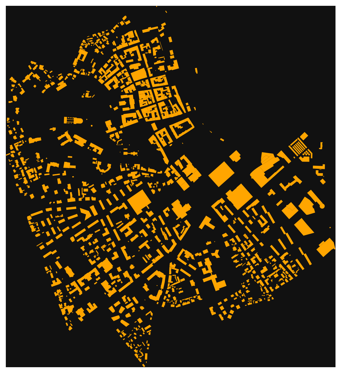
Nice! Now, as we can see, we have our OSM data as GeoDataFrames and we can plot them using the same functions and tools as we have used before.
There are also other ways of retrieving the data from OpenStreetMap with osmnx such as passing a Polygon to extract the data from that area, or passing a Point coordinates and retrieving data around that location with specific radius. Take a look at te developer tutorials to find out how to use those features of osmnx.
Let's create a map out of the streets and buildings but again exclude the nodes (to keep the figure clearer).
buildings_3301 = gdf_proj.to_crs(3301)

plt.style.use('dark_background')

fig, ax = plt.subplots(figsize=(10,8))

streets_3301.plot(ax=ax, linewidth=2, alpha=0.9, column='speed', cmap='Greens_r')
buildings_3301.plot(ax=ax, lw=4, edgecolor='lightgreen', facecolor='white', alpha=0.8)

plt.show()

# make sure to reset matplotlib style again
plt.style.use('default')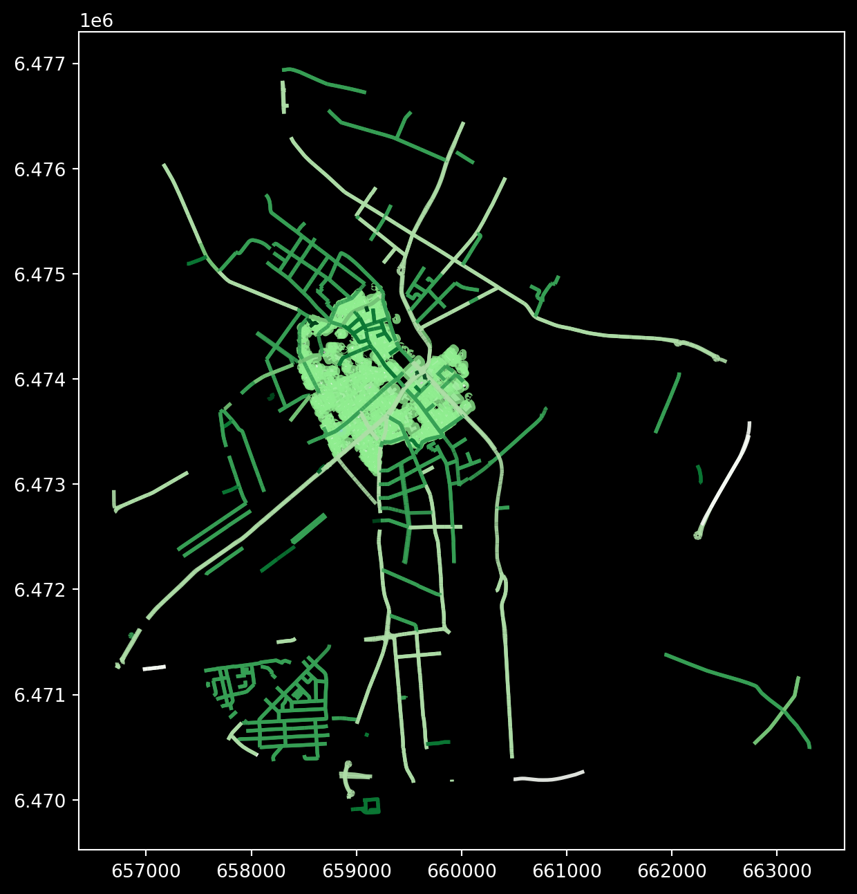
Cool! Now we have a map where we have plotted the buildings, streets and the boundaries of the selected region of 'Tartu' in City Centre. And all of this required only a few lines of code.
Try following task yourself - Explore the column highway in our edges GeoDataFrame, it contains information about the type of the street (such as primacy, cycleway or footway). Select the streets that are walkable or that can be used with cycle and visualize only them with the buildings and the area polygon. Use different colors and line widths for the cycleways and footways.
There are a few nice and convenient high-level functions in osmnx that can be used to produce nice maps directly just by using a single function that might be useful. If you are interested take a look of this tutorial. In the lesson we won't cover these, because we wanted to keep as much control to ourselves as possible, hence using lower-level functions.
From OSM we loaded comparatively static geographic data. Now we want to throw in some spatio-temporal data into the mix.
In this lesson's data package is an export of a dataset from the Tartu City Government's open data portal. If you haven't downloaded the data yet, you can download (and then extract) the dataset zip-package from this link.
Originally, the dataset can only be accessed via a webservice API. This is an excerpt for the weeks 2021-03-02 to 2021-04-06 and contains traffic counter data, in 15 minute intervals for several streets and intersections in central Tartu - it counts the amounts of cars passing through. At the end of the lesson is an example how to access the API live with Python. But the time being let's use the exported data now.
Download the next file from here.
import geopandas as gpd
traffic_data = gpd.read_file('tartu_export_5km_buffer_week.gpkg', driver="GPKG", layer="liiklus")

traffic_data.head(3)
/usr/lib64/python3.13/site-packages/pyogrio/raw.py:198: RuntimeWarning: driver GPKG does not support open option DRIVER
return ogr_read(| name | count | lane | objectid | time | text_time | geometry | |
|---|---|---|---|---|---|---|---|
| 0 | LKL_Tiksoja | 1 | 2 | 296992 | 1616452200041 | 2021-03-22 22:30:00 | POINT (26.65439 58.40841) |
| 1 | LKL_Roopa | 17 | 1 | 296993 | 1616435100041 | 2021-03-22 17:45:00 | POINT (26.69739 58.34843) |
| 2 | LKL_Tiksoja | 3 | 2 | 296994 | 1616455800041 | 2021-03-22 23:30:00 | POINT (26.65439 58.40841) |
display(traffic_data.info())

display(traffic_data.describe())
<class 'geopandas.geodataframe.GeoDataFrame'>
RangeIndex: 30000 entries, 0 to 29999
Data columns (total 7 columns):
# Column Non-Null Count Dtype
--- ------ -------------- -----
0 name 30000 non-null object
1 count 30000 non-null int64
2 lane 30000 non-null int64
3 objectid 30000 non-null int64
4 time 30000 non-null int64
5 text_time 30000 non-null object
6 geometry 30000 non-null geometry
dtypes: geometry(1), int64(4), object(2)
memory usage: 1.6+ MBNone| count | lane | objectid | time | |
|---|---|---|---|---|
| count | 30000.000000 | 30000.000000 | 30000.000000 | 3.000000e+04 |
| mean | 30.813167 | 1.500467 | 320426.927500 | 1.615854e+12 |
| std | 33.594990 | 0.500008 | 17831.580679 | 8.779583e+08 |
| min | 0.000000 | 1.000000 | 296864.000000 | 1.614649e+12 |
| 25% | 3.000000 | 1.000000 | 304459.750000 | 1.614875e+12 |
| 50% | 19.000000 | 2.000000 | 311959.500000 | 1.616287e+12 |
| 75% | 51.000000 | 2.000000 | 340661.250000 | 1.616500e+12 |
| max | 436.000000 | 2.000000 | 348907.000000 | 1.617730e+12 |
The time field is currently a text field. Pandas supports proper datetime indexing and querying, so we want to convert the current string object into a datetime datatype. The easiest is to delegate the hard work of guessing snd trying the right format to 'pandas':
import pandas as pd

traffic_data['datetime'] = traffic_data['text_time'].apply(pd.to_datetime, infer_datetime_format=True )
/tmp/ipykernel_519/2602662204.py:3: UserWarning: The argument 'infer_datetime_format' is deprecated and will be removed in a future version. A strict version of it is now the default, see https://pandas.pydata.org/pdeps/0004-consistent-to-datetime-parsing.html. You can safely remove this argument.
traffic_data['datetime'] = traffic_data['text_time'].apply(pd.to_datetime, infer_datetime_format=True )For the 'time' column you could guess that it might look like an epoch time stamp. In general, at some point it makes sense to get more familiar with Python's datetime functions and Pandas datetime indexing and parsing support. Then you could try to parse it as a datetime timestamp, like so:
traffic_data['datetime'] = pd.to_datetime(traffic_data['time'], unit='ms')For a moment, you might have considered to use the chronological timestamps as an index, like for a time-series for a weather station? But in this example we can't do that because technically each location is its own separate time-series, and right now we don't even know how many distinct locations (in terms of identical Point geometries) we have.
As we have little knowledge about the dataset, we should try to get a feeling of value ranges, categories, times etc. For example, let's check how many different names there are. Maybe it gives us a clue as to what the spatial spread might be:
stations = len(traffic_data['name'].unique())
print(stations)
print(traffic_data['name'].value_counts())
16
name
LKL_Voru 1885
LKL_Narva_mnt 1881
LKL_Ilmatsalu 1881
LKL_Riia_mnt_LV 1880
LKL_Roomu 1880
LKL_Arukula 1879
LKL_Riia_mnt_LS 1876
LKL_Viljandi_mnt 1876
LKL_Rapina_mnt 1874
LKL_Tiksoja 1873
LKL_Ringtee_3 1872
LKL_Lammi 1871
LKL_Ihaste 1871
LKL_Ringtee_2 1871
LKL_Ringtee_1 1868
LKL_Roopa 1862
Name: count, dtype: int64Officially a handful of distinct names. something we could now explore further as one way of aggregation. Let's look at the value distribution per "name" class. While the classic "Matplotlib" has the whole toolbox to plot whatever you desire or imagine, sometimes it is nice to use some higher level packages so we don't have to do all the coding by hand. Let me introduce to you the Seaborn package. Seaborn builds on top of the Python statistical and scientific ecosystem, and of course on top of Matplotlib, and provides a large number of high-quality and practical statistical plots and works nicely with dataframes. In the following image we are using a BoxPlot.
import seaborn as sns
import matplotlib.pyplot as plt
import matplotlib as mpl

mpl.rcParams['savefig.transparent'] = False
mpl.rcParams['savefig.facecolor'] = "w"

sns.set(rc={'figure.facecolor':'white'})

fig, ax = plt.subplots(figsize=(10,8))

sns.boxplot(x='name', y='count', data=traffic_data, ax=ax)

plt.title(f"Boxplot of Traffic Count values for different location names", fontsize='x-large')
plt.xticks(rotation=45, fontsize='large')
plt.xlabel("location name", fontsize='x-large')
plt.yticks(fontsize='large')
plt.ylabel("count", fontsize='x-large')

plt.show()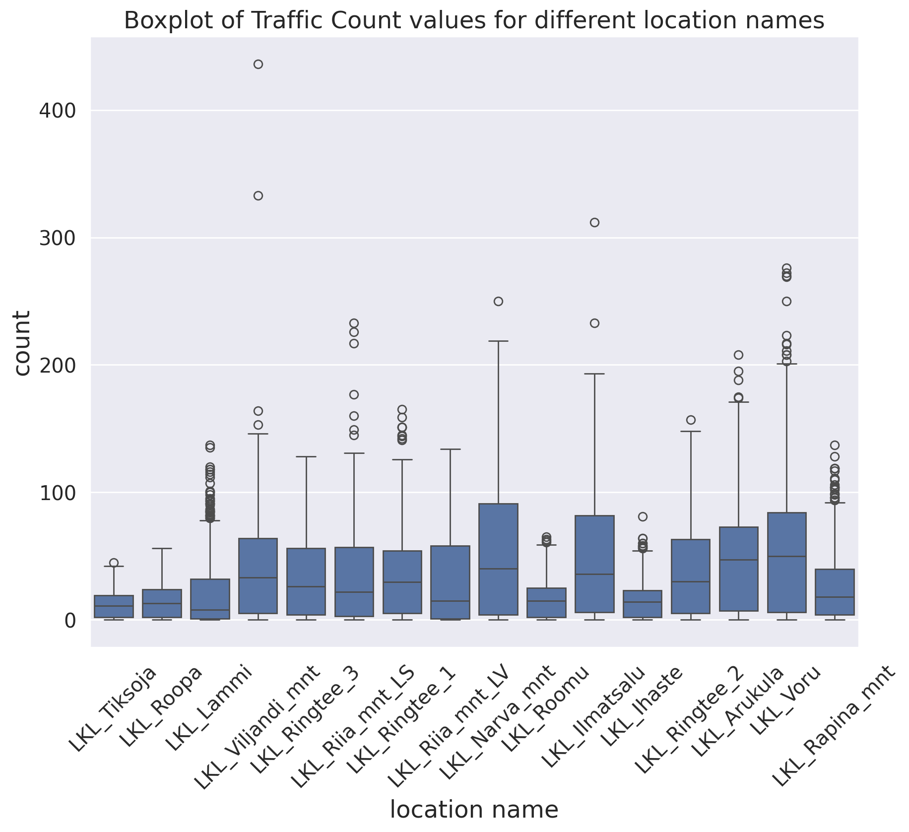
It looks like the traffic counters at Narva street have a wider variation then most. Let's explore only the counts for one "name" class for now. Later we can go back and apply the functions the whole dataset.
narva_lk = traffic_data.loc[traffic_data['name'] == "LKL_Narva_mnt"].copy()

fig, ax = plt.subplots(figsize=(10,8))

sns.histplot(data=narva_lk, x="count", ax=ax)
plt.title(f"Histogram of Traffic Count values for Narva Maantee location", fontsize='x-large')

plt.show()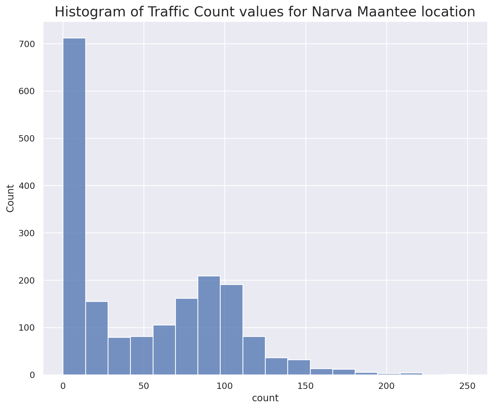
The histogram above shows the general distribution of measurement values, obviously, in most cases there are none or only very few cars measured per time interval. Let's make an aggregation for the hour of the day. Overall all days, take "sum()" for all counts that are during the same time of the day.
narva_lk['hour_of_day'] = narva_lk['datetime'].apply(lambda dtx: dtx.hour)
agg_narva_hours = []

for hod, sub_df in narva_lk.groupby(by='hour_of_day'):
    all_counts = sub_df['count'].sum()
    agg_narva_hours.append( { 'hod': hod, 'count': all_counts}  )

nava_hod_sum_df = pd.DataFrame(agg_narva_hours).set_index('hod')
nava_hod_sum_df.plot(kind='bar')

plt.title(f"Bar plot of the sum of Traffic Count values for the Narva Maantee location, per hour of the day", fontsize=12)

plt.show()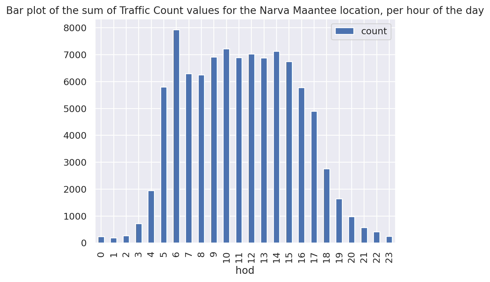
This is a bit easier, when you start getting more used to grouping and aggregating. You can write this now for the "average" (mean) in one line:
narva_lk.groupby(by='hour_of_day')['count'].mean().plot(kind='bar')
plt.title(f"Bar plot of the mean of Traffic Count values for the Narva Maantee location, per hour of the day", fontsize=12)

plt.show()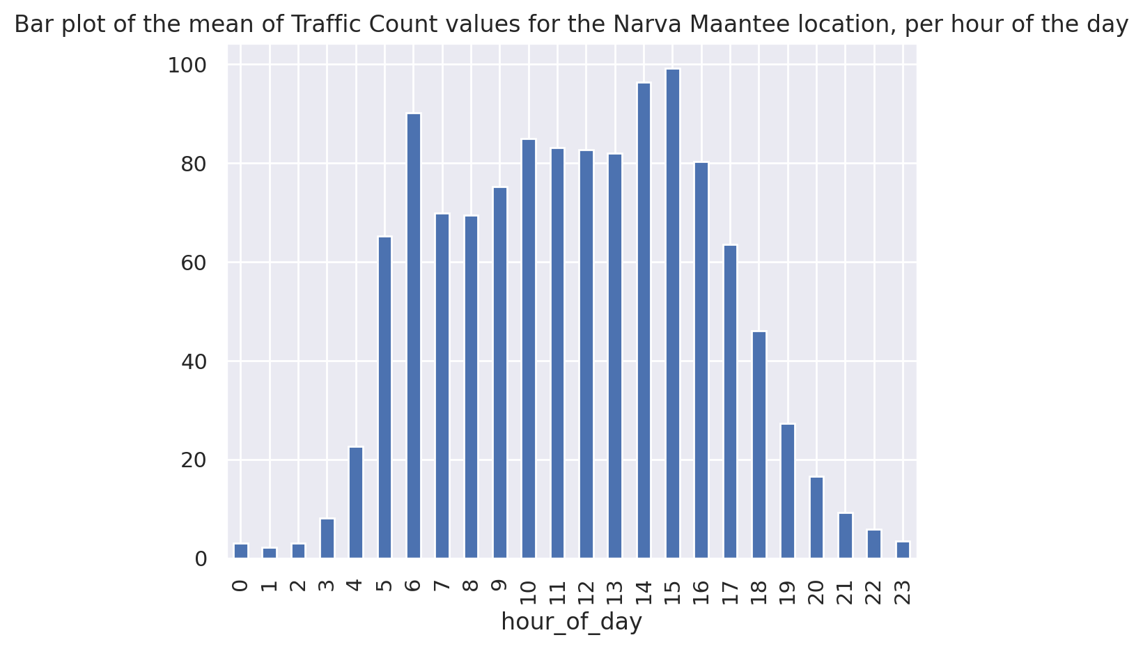
In the same way we should now also look at the weekday pattern.
narva_lk['day_of_week'] = narva_lk['datetime'].apply(lambda dtx: dtx.day_of_week)

fig, (ax_a, ax_b) = plt.subplots(1, 2, figsize=(10,8))
narva_lk.groupby(by='day_of_week')['count'].sum().plot(kind='bar', ax=ax_a)
narva_lk.groupby(by='day_of_week')['count'].mean().plot(kind='bar', ax=ax_b)

plt.show()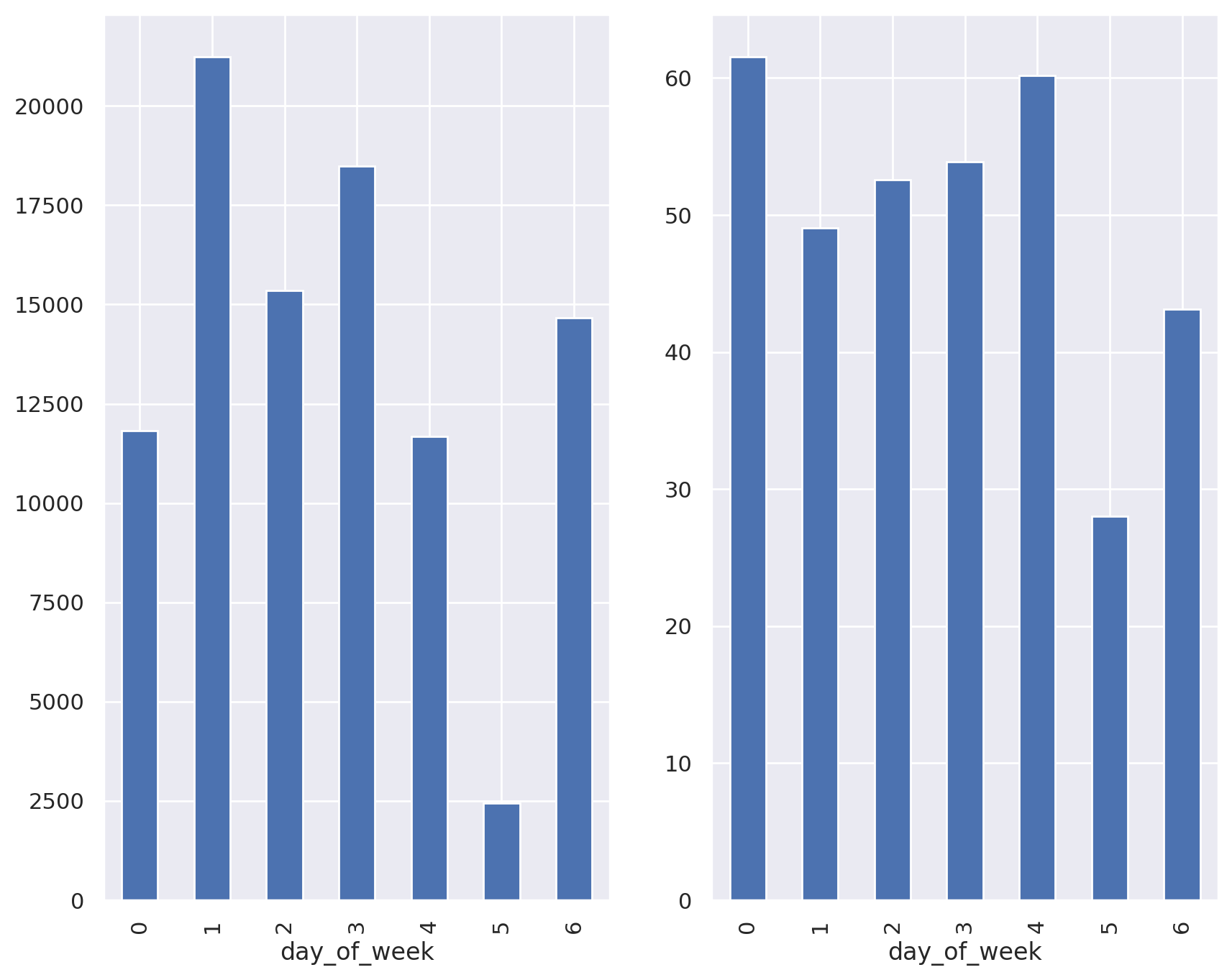
Now we have drilled down into the data quite a bit. Now let's figure out the spatial characteristics of the Narva station data.
print(len(narva_lk['geometry'].unique() ))6Although they share the same station name, there are still a few different geometries in this data slice. However, we can't aggregate directly on the Shapely geometry object type. But we know we can aggregate/groupby on strings. So now we use the WKT geometry text representation in order to group on those.
Shapely support loading and "dumping" geometries in WKT format.
narva_lk['wkt'] = narva_lk['geometry'].apply(lambda g: g.wkt)
narva_lk.groupby(by='wkt')['count'].mean().plot(kind='bar')

plt.show()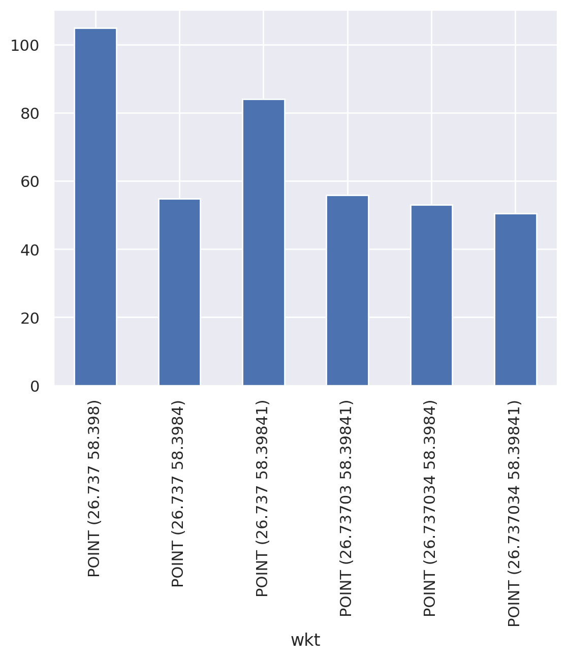
Let's now apply the steps on the whole dataset in order to make a map to visualise the traffic counts in Tartu on Tuesdays. At first we create our "day of week" column, and only subselect the observations for tuesdays (day=1). Secondly, we "destructure" our geometries to WKT for the spatial aggregation. We could potentially also use the station name, if we could agree that the single points are too close to each other to be meaningfully visualised separately.
traffic_data['day_of_week'] = traffic_data['datetime'].apply(lambda dtx: dtx.day_of_week)

tuesday_traffic = traffic_data.loc[traffic_data['day_of_week'] == 1].copy()
tuesday_traffic['wkt'] = tuesday_traffic['geometry'].apply(lambda g: g.wkt)
Now we will groupby WKT (i.e. location) at first, then take the mean for all observations at a single point (the location), and the mean represent the average of counts on all Tuesdays. We rejoin them into a separate geodataframe which we need to reproject into EPSG:3301 (Estonia) to plotted together with our OSM urban data from above.
from shapely import wkt
agg_traffic_day = []

for geom, sub_df in tuesday_traffic.groupby(by='wkt'):
    all_counts = sub_df['count'].mean()
    name = sub_df['name'].to_list()[0]
    agg_traffic_day.append( { 'name': name, 'count': all_counts, 'geometry': wkt.loads(geom)}  )

tues_agg = pd.DataFrame(agg_traffic_day)
tues_agg_3301 = gpd.GeoDataFrame(tues_agg, geometry='geometry', crs=4326).to_crs(3301)
Finally, we put the layers together in a single plot. The traffic counters seem to be distributed rather around the city than within.
plt.style.use('dark_background')

fig, ax = plt.subplots(figsize=(10,8))

streets_3301.plot(ax=ax, linewidth=2, alpha=0.9, color="gray", zorder=1)
streets_3301.plot(ax=ax, linewidth=2, alpha=0.9, column='speed', cmap='Greens_r', zorder=3)

tues_agg_3301.plot(ax=ax, markersize=150, edgecolor='gray', lw=1, column="count", cmap="Reds", alpha=0.8, legend=True, zorder=5)

plt.title("Average traffic flow (number cars passing) on Tuesdays during March 2021")

plt.show()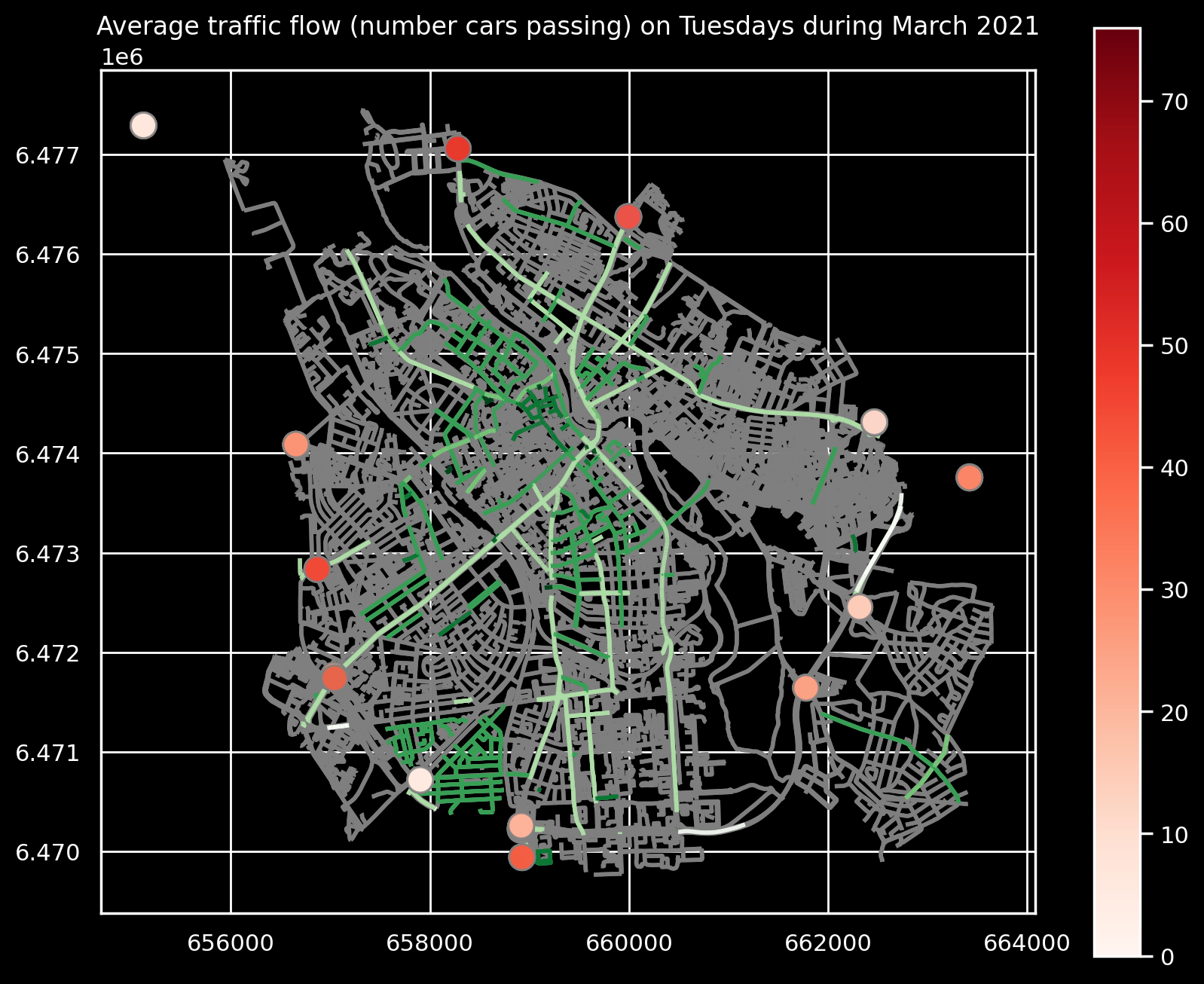
# reset some stuff again
import matplotlib.pyplot as plt
import matplotlib as mpl

mpl.rcParams.update(mpl.rcParamsDefault)
plt.style.use('default')

# plt.close('all')WarningThis code block shows an example of how to access the data. Use with care, don't overload the server with unbounded queries, such as too larger time spans for example. There are different query patterns possible as well, such as via envelope/bbox.
import requests
import datetime

query_url = "https://gis.tartulv.ee/arcgis/rest/services/Hosted/LiiklusloendLaneBigDatastoreView/FeatureServer/0/query"

starttime = datetime.datetime(2021, 10, 4, 0, 0, 0)
endtime = datetime.datetime(2021, 10, 10, 23, 59, 59)
ts1 = int(starttime.timestamp()) * 1000
ts2 = int(endtime.timestamp()) * 1000

# available fields = "name":"LKL_Roomu","count":13,"globalid1":"{B253DBFB-8596-F347-7873-D9C433520079}","latitude":58.378952,"lane":1,"objectid":297054,"globalid":6.5485272E8,"longitude":26.777779,"time":1616432400041

params = {'f': 'geojson','returnGeometry': 'true', 'resultRecordCount': 40, 'where': "name='LKL_Roomu'", "time":"{t1}, {t2}", "outFields": "objectid,name,lane,count,time"}

req = requests.get(query_url, params=params)

import geopandas as gpd
gdata = req.json()

gdf = gpd.GeoDataFrame.from_features(gdata['features'])
gdf.crs = "EPSG:4326"