Spatial modelling with Random Forest

Virro, H., Jemeljanova, M., Chan, W.T., Kmoch, A., Uuemaa, E.

Landscape Geoinformatics Lab, Department of Geography, University of Tartu

https://landscape-geoinformatics.ut.ee/

Preface

Machine learning has been increasingly used due to its capability to work with large amounts of data while having minimal assumptions on the distribution of variables. There are different types of machine learning and the figure below gives a brief overview of types of machine learning (Figure 1).

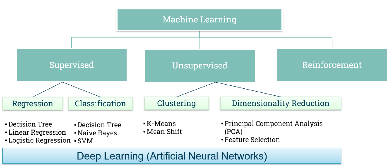
Figure 1. Types of machine learning

Random Forest is one of the most common machine learning algorithms (Breiman, 2001). We will also use Random Forest in this lesson. Random Forest is used for both classification and regression. It works by building multiple decision trees on different random subsets of the data and features.

Decision trees split data to create purer groups regarding the target variable. Purity means how homogenous the resulting groups are. This is optimized at each split by maximizing purity (or minimizing impurity). Impurity (the opposite of purity) is measured by metrics like entropy (disorder) or the Gini Index (likelihood of incorrect labelling). Alternatively, splits aim to maximize information gain, which is the reduction in entropy after a split. Higher information gain indicates a better split (Figure 2).

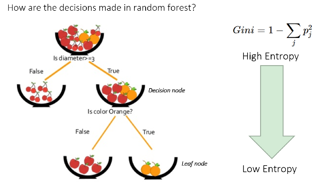
Figure 2. Overview of how decisions are made in Random Forest model. Source: Simplilearn

For a prediction, it averages the predictions of all the trees (for regression) or takes a majority vote (for classification). This “forest” of randomly created trees is more robust and less prone to overfitting than a single decision tree (Figure 3).

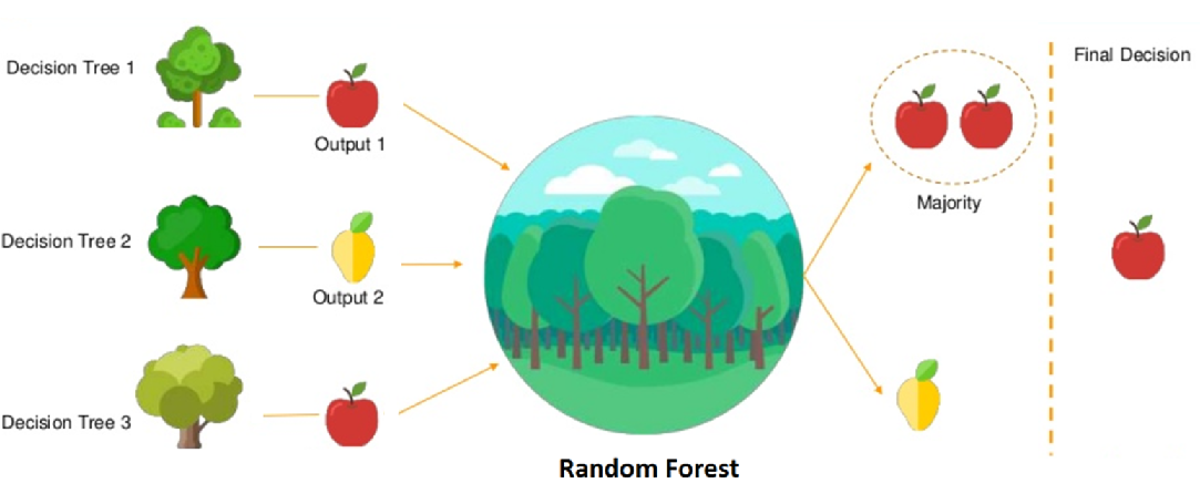
Figure 3. Overview of how final prediction is being made across all the trees. Source: Simplilearn

Machine learning models are often considered a black-box, and a lack of interpretability would mean that it is hard to determine if the model has found meaningful and realistic relationships between different phenomena. Thus, there is a strong need to be able to explain and interpret machine-learning models to understand the effects and relationships of the underlying modelled processes and used covariates.

Various methods to interpret the relationships between the covariates and the target variable in machine learning have been introduced (see, e.g, Molnar 2025). In this lesson, we cover some of the methods, namely partial dependence plots and Shapley values, and provide tips on how to make use of these methods to build less biased, better understandable, and more robust models.

In this lesson, we will use an example of predicting the total nitrogen (mg/L) in Estonian streams using various environmental variables (topography, soil, land use and land cover, hydrology, agriculture, and climate) calculated on the catchments of the respective streams (Figure 4) (see the details in Virro et al. 2022). The total nitrogen data was obtained from the KESE (Estonian Environmental Agency, 2021) environment monitoring system website maintained by the Estonian Environment Agency and was the average value between years 2016 and 2020. This lesson is adapted from the study “Random forest-based modelling of stream nutrients at national level in a data-scarce region” authored by Virro et al. (2022).

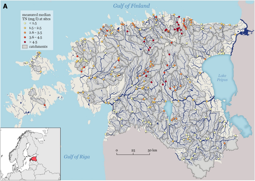
Figure 4. Total nitrogen monitoring points in Estonia

1. Dependences/ Library Import

Let’s import the packages. For the data processing, we will use numpy and pandas, to read in geospatial data, geopandas will be used. scikit-learn will be used for Random Forest modelling, shap for shap value calculation and plotting.The partial dependence plots will be generated with scikit-learn’s PartialDependenceDisplay function. Seaborn and matplotlib will be used for plotting.

Make sure that those packages have been installed in the geopython environment - scikit-learn - joblib - shap

# conda or micromamba in your geopython2025 activated environment
micromamba install -c conda-forge scikit-learn joblib shap

# Import packages
import seaborn as sns
import numpy as np
import geopandas as gpd
from sklearn.model_selection import train_test_split, RandomizedSearchCV
from sklearn.ensemble import RandomForestRegressor
from joblib import dump, load
from sklearn.metrics import r2_score
import shap
import matplotlib.pyplot as plt
import pandas as pd
import random
from sklearn.metrics import mean_squared_error
from sklearn.inspection import PartialDependenceDisplay

sns.set_theme()

2. Prepare RF training and test sets

The prediction target (total nitrogen) and feature values (land use, soil etc) are in tn_mean_obs_sites.gpkg download here.

2.1 Data Exploration (very simple one)

Let’s explore the contents of the file. We will use the geopandas package, since has the capacity to read in and work with spatial data.

# Read observation data
fp = "tn_mean_obs_sites.gpkg"
obs_data = gpd.read_file(fp)
display(obs_data)

	site_code	obs_id	obs_value	arable_prop	arable_prop_buff_100	arable_prop_buff_1000	arable_prop_buff_500	area	awc1_min	awc1_max	...	tri_mean	tri_std	twi_min	twi_max	twi_mean	twi_std	urban_prop	water_prop	wetland_prop	geometry
0	SJA8127000	161	1.0288	0.086	0.175	0.092	0.124	1.512569e+08	0.178	0.212	...	0.119	0.176	2.206	14.725	9.732	1.706	0.006	0.005	0.129	POINT (696315 6546937)
1	SJA9900000	200	1.3402	0.182	0.170	0.178	0.190	8.071414e+08	0.173	0.215	...	0.100	0.191	1.725	15.356	9.827	1.375	0.026	0.008	0.087	POINT (669868 6591973)
2	SJA3956000	90	6.6156	0.536	0.340	0.520	0.464	4.229881e+08	0.169	0.207	...	0.112	0.150	1.869	15.563	9.910	1.513	0.049	0.003	0.006	POINT (636008 6603086)
3	SJA1934000	40	1.6676	0.243	0.134	0.172	0.156	2.132077e+08	0.173	0.211	...	0.109	0.183	1.842	14.976	9.745	1.348	0.056	0.004	0.014	POINT (700294 6592517)
4	SJA7837000	157	2.8696	0.293	0.321	0.330	0.352	3.100426e+08	0.173	0.208	...	0.111	0.151	1.859	15.576	9.724	1.397	0.111	0.007	0.058	POINT (520653 6588232)
...	...	...	...	...	...	...	...	...	...	...	...	...	...	...	...	...	...	...	...	...	...
234	SJB3503000	238	8.2250	0.537	0.316	0.523	0.453	1.122941e+08	0.174	0.205	...	0.099	0.111	2.279	15.563	10.033	1.392	0.028	0.002	0.014	POINT (633230 6585334)
235	SJA3731000	84	1.7250	0.200	0.065	0.122	0.085	6.085978e+07	0.175	0.206	...	0.124	0.223	1.842	14.565	9.663	1.395	0.072	0.003	0.009	POINT (698754 6586118)
236	SJA0813000	17	3.2500	0.452	0.223	0.499	0.475	4.023375e+07	0.174	0.207	...	0.207	0.272	2.373	16.631	9.019	2.097	0.033	0.007	0.014	POINT (619933 6581023)
237	SJA8884000	175	3.3000	0.242	0.176	0.232	0.225	1.930663e+09	0.164	0.218	...	0.105	0.145	1.464	15.329	9.728	1.468	0.025	0.010	0.106	POINT (551221 6591443)
238	SJA1953000	41	3.0050	0.479	0.266	0.498	0.455	9.860328e+07	0.172	0.207	...	0.178	0.246	2.294	16.631	9.266	1.959	0.028	0.004	0.027	POINT (619319 6581605)

239 rows × 86 columns

In machine learning the value that you want to predict is called target value and the predictors are called features or covariates. In our case, the prediction target is obs_value - total nitrogen (mg/l) the predictor variables aka features are all the features between the obs_value (82 features), and the geometry, where the spatial information is stored.

Altogether, we have 239 observations (samples) from which we can build a machine learning model. Random Forests, like most machine learning algorithms, typically benefit from having more training data. With more data, the Random Forest can potentially capture more complex and nuanced relationships in the data without overfitting. However, the benefit of adding more data eventually diminishes. Once the model has learned the underlying patterns sufficiently, adding significantly more data might only lead to marginal improvements in performance. Moreover, the quality and relevance of the data are often more important than just the quantity.

In general, random forest works best on quantitative data, but you can also add qualitative data into the model. However, qualitative data needs to be converted into dummy variables (binary - 0 or 1). Before modelling, we should check our data types.

#Check the data type of the features and the target
obs_data.info()

<class 'geopandas.geodataframe.GeoDataFrame'>
RangeIndex: 239 entries, 0 to 238
Data columns (total 86 columns):
 #   Column                         Non-Null Count  Dtype   
---  ------                         --------------  -----   
 0   site_code                      239 non-null    object  
 1   obs_id                         239 non-null    int64   
 2   obs_value                      239 non-null    float64 
 3   arable_prop                    239 non-null    float64 
 4   arable_prop_buff_100           239 non-null    float64 
 5   arable_prop_buff_1000          239 non-null    float64 
 6   arable_prop_buff_500           239 non-null    float64 
 7   area                           239 non-null    float64 
 8   awc1_min                       239 non-null    float64 
 9   awc1_max                       239 non-null    float64 
 10  awc1_mean                      239 non-null    float64 
 11  awc1_std                       239 non-null    float64 
 12  bd1_min                        239 non-null    float64 
 13  bd1_max                        239 non-null    float64 
 14  bd1_mean                       239 non-null    float64 
 15  bd1_std                        239 non-null    float64 
 16  clay1_min                      239 non-null    float64 
 17  clay1_max                      239 non-null    float64 
 18  clay1_mean                     239 non-null    float64 
 19  clay1_std                      239 non-null    float64 
 20  dem_min                        239 non-null    float64 
 21  dem_max                        239 non-null    float64 
 22  dem_mean                       239 non-null    float64 
 23  dem_std                        239 non-null    float64 
 24  flowlength_min                 239 non-null    float64 
 25  flowlength_max                 239 non-null    float64 
 26  flowlength_mean                239 non-null    float64 
 27  flowlength_std                 239 non-null    float64 
 28  forest_disturb_prop_buff_100   239 non-null    float64 
 29  forest_disturb_prop_buff_1000  239 non-null    float64 
 30  forest_disturb_prop_buff_500   239 non-null    float64 
 31  forest_prop                    239 non-null    float64 
 32  grassland_prop                 239 non-null    float64 
 33  k1_min                         239 non-null    float64 
 34  k1_max                         239 non-null    float64 
 35  k1_mean                        239 non-null    float64 
 36  k1_std                         239 non-null    float64 
 37  limestone_prop                 239 non-null    float64 
 38  livestock_density              239 non-null    float64 
 39  manure_dep_n                   239 non-null    float64 
 40  manure_dep_p                   239 non-null    float64 
 41  other_prop                     239 non-null    float64 
 42  pol_sen_drain_h_prop           239 non-null    float64 
 43  pol_sen_drain_vh_prop          239 non-null    float64 
 44  pol_sen_nat_h_prop             239 non-null    float64 
 45  pol_sen_nat_vh_prop            239 non-null    float64 
 46  precip_mean                    239 non-null    float64 
 47  rip_veg_drain_prop             239 non-null    float64 
 48  rip_veg_nat_prop               239 non-null    float64 
 49  rock1_min                      239 non-null    float64 
 50  rock1_max                      239 non-null    float64 
 51  rock1_mean                     239 non-null    float64 
 52  rock1_std                      239 non-null    float64 
 53  sand1_min                      239 non-null    float64 
 54  sand1_max                      239 non-null    float64 
 55  sand1_mean                     239 non-null    float64 
 56  sand1_std                      239 non-null    float64 
 57  silt1_min                      239 non-null    float64 
 58  silt1_max                      239 non-null    float64 
 59  silt1_mean                     239 non-null    float64 
 60  silt1_std                      239 non-null    float64 
 61  slope_min                      239 non-null    float64 
 62  slope_max                      239 non-null    float64 
 63  slope_mean                     239 non-null    float64 
 64  slope_std                      239 non-null    float64 
 65  snow_depth_mean                239 non-null    float64 
 66  soc1_min                       239 non-null    float64 
 67  soc1_max                       239 non-null    float64 
 68  soc1_mean                      239 non-null    float64 
 69  soc1_std                       239 non-null    float64 
 70  stream_density                 239 non-null    float64 
 71  temp_max                       239 non-null    float64 
 72  temp_mean                      239 non-null    float64 
 73  temp_min                       239 non-null    float64 
 74  tri_min                        239 non-null    float64 
 75  tri_max                        239 non-null    float64 
 76  tri_mean                       239 non-null    float64 
 77  tri_std                        239 non-null    float64 
 78  twi_min                        239 non-null    float64 
 79  twi_max                        239 non-null    float64 
 80  twi_mean                       239 non-null    float64 
 81  twi_std                        239 non-null    float64 
 82  urban_prop                     239 non-null    float64 
 83  water_prop                     239 non-null    float64 
 84  wetland_prop                   239 non-null    float64 
 85  geometry                       239 non-null    geometry
dtypes: float64(83), geometry(1), int64(1), object(1)
memory usage: 160.7+ KB

#check the all the column names aka features
obs_data.columns

Index(['site_code', 'obs_id', 'obs_value', 'arable_prop',
       'arable_prop_buff_100', 'arable_prop_buff_1000', 'arable_prop_buff_500',
       'area', 'awc1_min', 'awc1_max', 'awc1_mean', 'awc1_std', 'bd1_min',
       'bd1_max', 'bd1_mean', 'bd1_std', 'clay1_min', 'clay1_max',
       'clay1_mean', 'clay1_std', 'dem_min', 'dem_max', 'dem_mean', 'dem_std',
       'flowlength_min', 'flowlength_max', 'flowlength_mean', 'flowlength_std',
       'forest_disturb_prop_buff_100', 'forest_disturb_prop_buff_1000',
       'forest_disturb_prop_buff_500', 'forest_prop', 'grassland_prop',
       'k1_min', 'k1_max', 'k1_mean', 'k1_std', 'limestone_prop',
       'livestock_density', 'manure_dep_n', 'manure_dep_p', 'other_prop',
       'pol_sen_drain_h_prop', 'pol_sen_drain_vh_prop', 'pol_sen_nat_h_prop',
       'pol_sen_nat_vh_prop', 'precip_mean', 'rip_veg_drain_prop',
       'rip_veg_nat_prop', 'rock1_min', 'rock1_max', 'rock1_mean', 'rock1_std',
       'sand1_min', 'sand1_max', 'sand1_mean', 'sand1_std', 'silt1_min',
       'silt1_max', 'silt1_mean', 'silt1_std', 'slope_min', 'slope_max',
       'slope_mean', 'slope_std', 'snow_depth_mean', 'soc1_min', 'soc1_max',
       'soc1_mean', 'soc1_std', 'stream_density', 'temp_max', 'temp_mean',
       'temp_min', 'tri_min', 'tri_max', 'tri_mean', 'tri_std', 'twi_min',
       'twi_max', 'twi_mean', 'twi_std', 'urban_prop', 'water_prop',
       'wetland_prop', 'geometry'],
      dtype='object')

Before diving into machine learning, it is always useful to run simple correlation analysis. If there is absolutely no correlation between the target variable and the features then usually machine learning would also not work. Let’s create correlation matrix.

# Calculate the correlation matrix
correlation_matrix = obs_data[['obs_value', 'arable_prop',
       'arable_prop_buff_100', 'arable_prop_buff_1000', 'arable_prop_buff_500',
       'area', 'awc1_min', 'awc1_max', 'awc1_mean', 'awc1_std', 'bd1_min',
       'bd1_max', 'bd1_mean', 'bd1_std', 'clay1_min', 'clay1_max',
       'clay1_mean', 'clay1_std', 'dem_min', 'dem_max', 'dem_mean', 'dem_std',
       'flowlength_min', 'flowlength_max', 'flowlength_mean', 'flowlength_std',
       'forest_disturb_prop_buff_100', 'forest_disturb_prop_buff_1000',
       'forest_disturb_prop_buff_500', 'forest_prop', 'grassland_prop',
       'k1_min', 'k1_max', 'k1_mean', 'k1_std', 'limestone_prop',
       'livestock_density', 'manure_dep_n', 'manure_dep_p', 'other_prop',
       'pol_sen_drain_h_prop', 'pol_sen_drain_vh_prop', 'pol_sen_nat_h_prop',
       'pol_sen_nat_vh_prop', 'precip_mean', 'rip_veg_drain_prop',
       'rip_veg_nat_prop', 'rock1_min', 'rock1_max', 'rock1_mean', 'rock1_std',
       'sand1_min', 'sand1_max', 'sand1_mean', 'sand1_std', 'silt1_min',
       'silt1_max', 'silt1_mean', 'silt1_std', 'slope_min', 'slope_max',
       'slope_mean', 'slope_std', 'snow_depth_mean', 'soc1_min', 'soc1_max',
       'soc1_mean', 'soc1_std', 'stream_density', 'temp_max', 'temp_mean',
       'temp_min', 'tri_min', 'tri_max', 'tri_mean', 'tri_std', 'twi_min',
       'twi_max', 'twi_mean', 'twi_std', 'urban_prop', 'water_prop',
       'wetland_prop']].corr()

# Set up the matplotlib figure
plt.figure(figsize=(10, 8))

# Create a heatmap using seaborn
sns.heatmap(correlation_matrix, cmap='coolwarm', fmt='.2f', square=True, 
            cbar_kws={"shrink": .8}, linewidths=0.5)

# Set titles and labels
plt.title('Correlation Matrix')
plt.xticks(rotation=90)  # Rotate x-axis labels for better readability
plt.yticks(rotation=0)    # Rotate y-axis labels for better readability

# Show the plot
plt.tight_layout()
plt.show()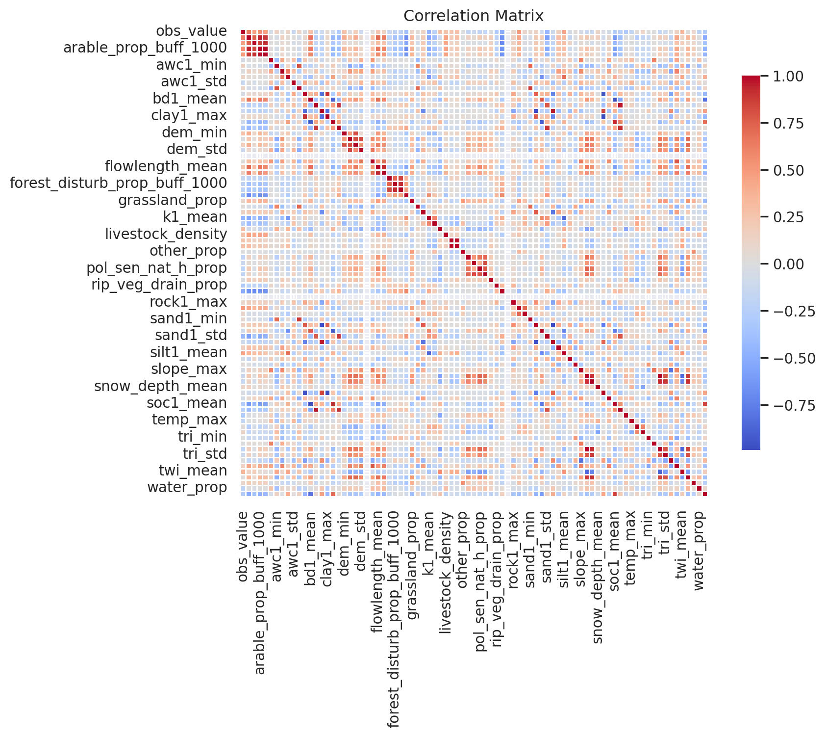

It is also useful to look at the histograms. Ideally target and all the features but for the simplicity, we will only look at the target and one variable (arable land proportion).

# Histograms of features
features = ['obs_value', 'arable_prop']
colors = ['skyblue', 'lightgreen']

# Create a figure with 3 subplots (1 row, 3 columns)
fig, axs = plt.subplots(1, 2, figsize=(18, 6))

# Loop through features to create histograms
for ax, feature, color in zip(axs, features, colors):
    obs_data[feature].hist(ax=ax, bins=30, color=color, edgecolor='black')
    ax.set_title(f'histogram of {feature}')  # Title in lowercase
    ax.set_xlabel(feature)                    # Axis label in lowercase
    ax.set_ylabel('frequency')                 # Axis label in lowercase

# Adjust layout
fig.tight_layout()

# Show the plots
plt.show()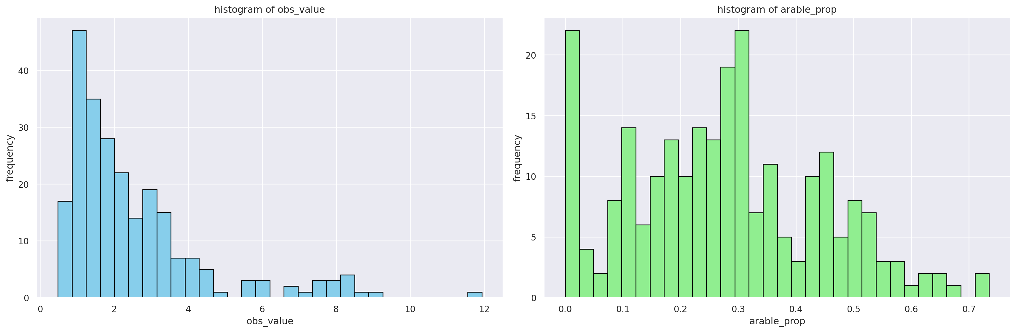

2.2 Data visualization

Let’s plot the data spatially, using the observed value of total nitrogen (mg/L).

# Create interactive plot of observation values
obs_data.explore(
    column="obs_value",
    cmap="YlOrRd",
    tooltip=["site_code", "obs_value"],
    marker_kwds={"radius": 4},
    style_kwds={"color": "black", "weight": 1, "fillOpacity": 0.9}
)

Make this Notebook Trusted to load map: File -> Trust Notebook

2.3 Training and testing dataset preparation

The first step of any modelling is to split your data into training and testing set. The primary goal of a machine learning model is to perform well on new, unseen data. Splitting the data into training and testing sets enables us to ensure that.

The training set is used to teach the model the patterns and relationships within the data. The model learns from this data and adjusts its internal parameters to minimize errors.

The testing set is a completely separate portion of the data that the model never sees during training. It’s used to evaluate the model’s performance on this new, unseen data. This provides a realistic estimate of how well the model will perform in the real world.

First, we will extract the features and the prediction target into separate variables. We will remove the id columns, the prediction target (first three columns), and the geometry column (the last column) from the training data, as they are not necessary for the model training. We will save the prediction target values separately. Throughout the workshop, we will use X to represent covariates (or features), and Y as the target variable.

# Extract features and target
X = obs_data.iloc[:, 3:-1] #takes columns between 3rd and the last column of the data frame
y = obs_data["obs_value"] #Lowercase y is conventionally used to represent the target variable (a 1D array or Series containing the values to be predicted).

Random Forest relies on randomisation (as the name implies) in subsetting data for decision trees. However, if we want to ensure reproducibility then we need our data split to be consistent. This is important when you want to fairly compare different models or different configurations of the same model and also if you’re sharing your code or results with others, setting a random_state allows them to run your script and obtain the exact same data split and therefore the same model training and evaluation outcomes.

Parameter random_state is controlling whether your split is random or not. in the way your data is split into training and testing sets.

If you don’t specify a random_state, the shuffling process will be different every time you run the script. This means that the exact composition of your training and testing sets will vary across different runs.

We will set the random_state to 42. The reason random_state is often set to 42 in machine learning (and programming in general) is primarily due to its status as a well-known and somewhat humorous “magic number” in popular culture, stemming from Douglas Adams’ science fiction series The Hitchhiker’s Guide to the Galaxy where the supercomputer Deep Thought calculates the “Answer to the Ultimate Question of Life, the Universe, and Everything” to be 42. :smile:

# Set the random_state
random_state = 42

Now we will split the dataset randomly into 70% training data and 30% testing data. We will create four different data frames for training and testing to ensure that the features correspond to the respective prediction targets.

# Split the data into training and test sets
test_size = 0.3
X_train, X_test, y_train, y_test = train_test_split(X, y, test_size=test_size, random_state=random_state)

If we now look at the X_train then we can see that we will train our model on 167 samples.

X_train

	arable_prop	arable_prop_buff_100	arable_prop_buff_1000	arable_prop_buff_500	area	awc1_min	awc1_max	awc1_mean	awc1_std	bd1_min	...	tri_max	tri_mean	tri_std	twi_min	twi_max	twi_mean	twi_std	urban_prop	water_prop	wetland_prop
29	0.351	0.170	0.358	0.333	930164575.0	0.000	0.211	0.187	0.005	0.000	...	12.076	0.168	0.202	0.673	15.615	9.081	1.748	0.030	0.009	0.064
124	0.448	0.222	0.359	0.318	220221100.0	0.174	0.220	0.197	0.004	0.412	...	922.779	0.086	0.449	0.157	15.460	10.148	1.329	0.023	0.002	0.027
75	0.348	0.231	0.347	0.327	9772100.0	0.167	0.203	0.192	0.006	0.421	...	4.070	0.345	0.304	2.222	14.906	7.579	2.124	0.034	0.051	0.045
82	0.215	0.159	0.217	0.202	97323725.0	0.177	0.213	0.197	0.004	0.408	...	2.368	0.085	0.090	2.167	14.672	9.923	1.150	0.012	0.001	0.022
5	0.089	0.114	0.090	0.101	591638725.0	0.174	0.219	0.196	0.006	0.372	...	4.234	0.083	0.137	1.821	15.492	9.941	1.226	0.008	0.005	0.150
...	...	...	...	...	...	...	...	...	...	...	...	...	...	...	...	...	...	...	...	...	...
106	0.012	0.016	0.013	0.014	29728700.0	0.179	0.198	0.190	0.002	0.407	...	1.600	0.087	0.084	2.933	13.654	9.331	0.928	0.032	0.005	0.102
14	0.316	0.163	0.308	0.268	300674675.0	0.167	0.207	0.190	0.005	0.373	...	4.090	0.143	0.211	2.207	16.631	9.605	1.804	0.021	0.005	0.080
92	0.295	0.282	0.341	0.312	86506875.0	0.180	0.212	0.196	0.004	0.394	...	5.666	0.104	0.134	1.745	14.406	9.651	1.401	0.050	0.007	0.170
179	0.042	0.106	0.083	0.122	90116275.0	0.165	0.202	0.190	0.005	0.419	...	2.018	0.061	0.053	2.549	13.705	9.795	0.883	0.003	0.001	0.301
102	0.017	0.057	0.017	0.021	4168925.0	0.182	0.194	0.190	0.002	0.421	...	1.094	0.089	0.079	4.362	12.555	9.332	0.908	0.136	0.002	0.087

167 rows × 82 columns

And we can also look at our target variable.

y_train

29     1.4770
124    3.2750
75     0.7220
82     3.0750
5      0.9756
        ...  
106    2.0000
14     3.7582
92     1.8700
179    1.1880
102    4.6500
Name: obs_value, Length: 167, dtype: float64

3. Hyperparameter tuning

Hyperparameters are configuration settings that are set before the machine learning model training process begins. They control various aspects of the learning algorithm and the structure of the model itself.

Hyperparameters are important because:

The ultimate goal of a machine learning model is to generalize well to unseen data. Properly tuned hyperparameters help to find the right balance between fitting the training data and generalizing to new data, minimizing overfitting and underfitting (Figure 5).
Hyperparameters can also impact the training time and resource requirements of a model. For example, a larger number of trees in a Random Forest will generally increase training time.
Hyperparameters determine the structure of the model. In a Random Forest, the n_estimators (number of trees) and max_depth (maximum depth of each tree) are hyperparameters that influence the model’s complexity. A model that is too simple (underfitting) might not capture the underlying patterns in the data, while a model that is too complex (overfitting) might learn the noise in the training data and perform poorly on new, unseen data.

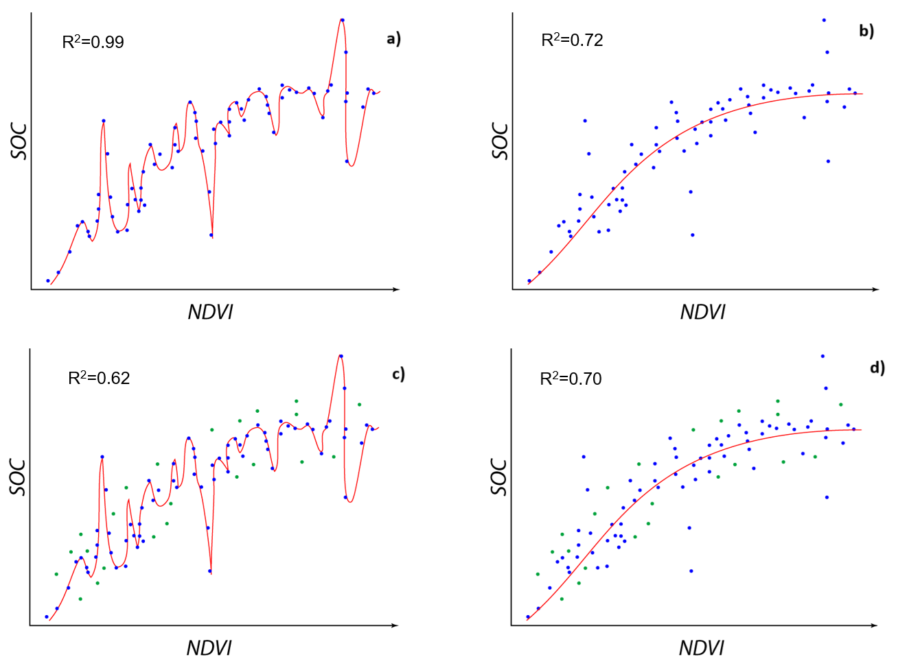
Figure 5. Overfitting: on a) and b) the R2 is better on a) but if we add new data (green points) then the initial model on a) becomes not so goon on c) and initial model b) is robust enough to be still good fitt for newly added points in d). The model a) is overfitted.

Before hyperparameter tuning, knowing which hyperparameters have the most significant impact is essential. For Random Forest, some of the most important ones include:

n_estimators: The number of trees in the forest. More trees usually improve accuracy and make the model more robust but also increase computation time. max_depth: The maximum depth of each decision tree. Limiting depth can help prevent overfitting. min_samples_split: The minimum number of samples required to split an internal node. Higher values can prevent overfitting. min_samples_leaf: The minimum number of samples required to be at a leaf node. Higher values can smooth the model and reduce overfitting. max_features: The number of features to consider when looking for the best split at each node. bootstrap: Whether bootstrap samples are used when building trees. criterion: The function used to measure the quality of a split (“gini” for classification, “squared_error” for regression). random_state: Controls the randomness of the training process for reproducibility.

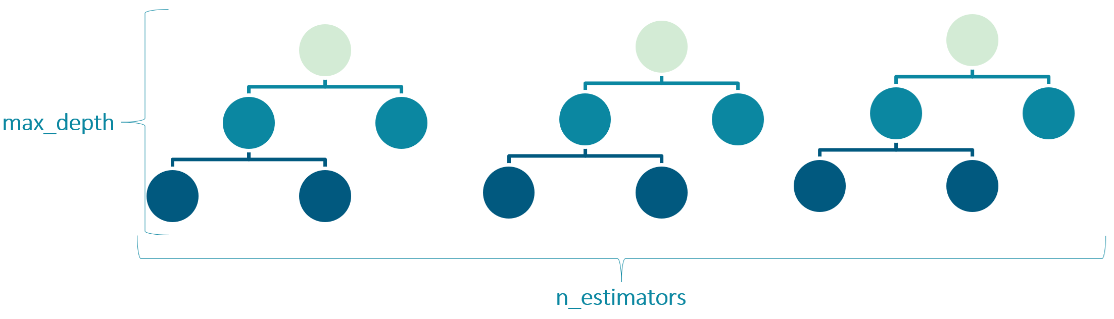
Figure 6. Hyperparameters n_estimators and max_depth for Random Forest.

There are several systematic ways to find the best combination of hyperparameters e.g. time consuming manual trial-error, randomized search, grid search, AutoML etc. It is recommended to start with the automatic methods (e.g., grid search or random search) and then manually check some parameters.

We will use the RandomisedSearchCV (Bergstra and Bengio, 2012) algorithm. We will define a list of possible hyperparameter values (value ranges), and the algorithm will determine which combination of them performs the best.

We will perform 100 runs (n_iter=100), and the best hyperparameter combination will be the one with the smallest resulting mean squared error (MSE) when running a model.

We will tune the following parameters:

n_estimators (number of trees in random forest);
max_depth (maximum number of levels in a tree)

# Search for hyperparameters
def search_hyperparams(X, y, random_state):

    # Number of trees in random forest - test between 50 to 200 with testing interval of 25
    step = 25
    n_estimators = list(np.arange(start=50, stop=200 + step, step=step))

    # Maximum number of levels in a tree - test between 5 and 20 with testing interval of 5
    step = 5
    max_depth = list(np.arange(start=5, stop=20 + step, step=step))

    # Create dictionary from parameters
    param_distributions = {
        "n_estimators": n_estimators,
        "max_depth": max_depth
    }

    # Perform search for hyperparameters
    estimator = RandomForestRegressor()
    rf_random = RandomizedSearchCV(
        estimator=estimator, #Specifies the model to tune (the RandomForestRegressor)
        param_distributions=param_distributions, 
        n_iter=100, #Specifies that RandomizedSearchCV will try 80 different random combinations of the hyperparameters.
        verbose=2, #Controls the verbosity of the search process, providing more detailed output during fitting.
        random_state=random_state, #Ensures that the random sampling of hyperparameter combinations is reproducible.
        n_jobs=-1 #Uses all available CPU cores to speed up the cross-validation process for each hyperparameter combination.
    )
    rf_random.fit(X, y)

    # Get best parameters
    params = rf_random.best_params_
    params["oob_score"] = True #passing manually the oob_score parameter to the params

    return params

%%time

# Perform search for hyperparameters
params = search_hyperparams(X_train, y_train, random_state)

Fitting 5 folds for each of 28 candidates, totalling 140 fits

/usr/lib64/python3.13/site-packages/sklearn/model_selection/_search.py:317: UserWarning: The total space of parameters 28 is smaller than n_iter=100. Running 28 iterations. For exhaustive searches, use GridSearchCV.
  warnings.warn(

CPU times: user 968 ms, sys: 436 ms, total: 1.4 s
Wall time: 9.44 s

# Show the best hyperparameters
params

{'n_estimators': np.int64(75), 'max_depth': np.int64(15), 'oob_score': True}

4. Model Training (with model parameters based on Hyperparameter tuning)

Now that we have the optimal hyperparameters, let’s train our model using them. First, we define the algorithm that we will use (Random Forest) and set the hyperparameters.

# Set the algorithm as Random Forest regressor and the hyperparameters from the previous step (params)
regressor = RandomForestRegressor(**params)

Next, we train (fit) the model on our feature and prediction target data.

# Fit model
regressor.fit(X_train, y_train)

RandomForestRegressor(max_depth=np.int64(15), n_estimators=np.int64(75),
                      oob_score=True)

In a Jupyter environment, please rerun this cell to show the HTML representation or trust the notebook.
On GitHub, the HTML representation is unable to render, please try loading this page with nbviewer.org.

Let’s see how well our model performed on the training data by calculating the R squared value. As R squared values span [0;1], where 1 means an ideal fit between the observations and predicted values and the value goes down as the model prediction gets worse.

# Calculate accuracy on training set
r2_training = regressor.score(X_train, y_train)
print(f"Training R-squared score: {r2_training:.2f}")

Training R-squared score: 0.94

However, looking at training R2 is very biased because model just predict on the data it was trained on. Correct thing to to is to look at either R2 on the testing data or OOB R2 (Out-of-Bag R-squared). R2 testing is the R2 that is being calculated on the 30% of the data that we initially left ut from the training set. OOB R2 (Out-of-Bag R-squared) is a performance metric specifically used for evaluating Random Forest regression models. It provides an estimate of how well the model generalizes to unseen data, similar to using a validation set, but without the need for a separate split of your training data.

How OOB R2 is calculated? For each decision tree in the forest, the data points that were not included in its specific bootstrap sample are called the out-of-bag (OOB) samples for that tree. Approximately 37% of the training data, on average, will be OOB for any given tree. Then OOB prediction is calculated for a specific data point considering only the trees in the Random Forest that did not use that data point in their training. All predictions of these trees are averaged for that particular data point. The OOB R2 is calculated by comparing the OOB predictions for all data points in the training set with their actual values.

# Calculate OOB R2
oob_r2 = regressor.oob_score_
print(f"OOB R-squared score: {oob_r2:.2f}")

OOB R-squared score: 0.55

# Predict
y_train_pred = regressor.predict(X_train)
y_test_pred = regressor.predict(X_test)

Let’s also determine the model generalisation capacity by determining R squared on independent data that the model has not seen (i.e., our test data). While the score is fair, it is lower than for the training data, meaning that there has been a fair bit of overfitting to the training data.

# Calculate accuracy on test set
r2_score(y_test, y_test_pred)

0.6292543438015875

In addition, one should always look at some error metrics. Let’s calculate OOB Mean Squared Error. It measures the average of the squared differences between the predicted OOB values and the actual (true) values.

# Calculate OOB Mean Squared Error (MSE) manually
oob_predictions = regressor.oob_prediction_
oob_mse = mean_squared_error(y_train, oob_predictions)
print(f"Out-of-Bag Mean Squared Error (OOB MSE): {oob_mse:.4f}")

Out-of-Bag Mean Squared Error (OOB MSE): 1.5990

We should also plot predicted vs. observed. If the predicted values closely follow a straight diagonal line (y = x), it indicates that the model’s predictions are very close to the observed values, suggesting good overall performance. It also enables to detect outliers - data points that are far from the diabonal line.

# Make predictions on the test set (or your entire dataset)
y_predicted = regressor.predict(X_test)
y_observed = y_test

# Create the plot
plt.figure(figsize=(9, 6))
plt.scatter(y_observed, y_predicted, color='blue', alpha=0.5)

# Add a diagonal line for perfect predictions
min_val = min(np.min(y_observed), np.min(y_predicted))
max_val = max(np.max(y_observed), np.max(y_predicted))
plt.plot([min_val, max_val], [min_val, max_val], color='red', linestyle='--')

# Add labels and title
plt.xlabel("Observed Values", fontsize=14)
plt.ylabel("Predicted Values", fontsize=14)
plt.title("Predicted vs. Observed Values - Test (Random Forest Regression)", fontsize=16)

# Add a grid for better readability
plt.grid(True)

# Show the plot
plt.show()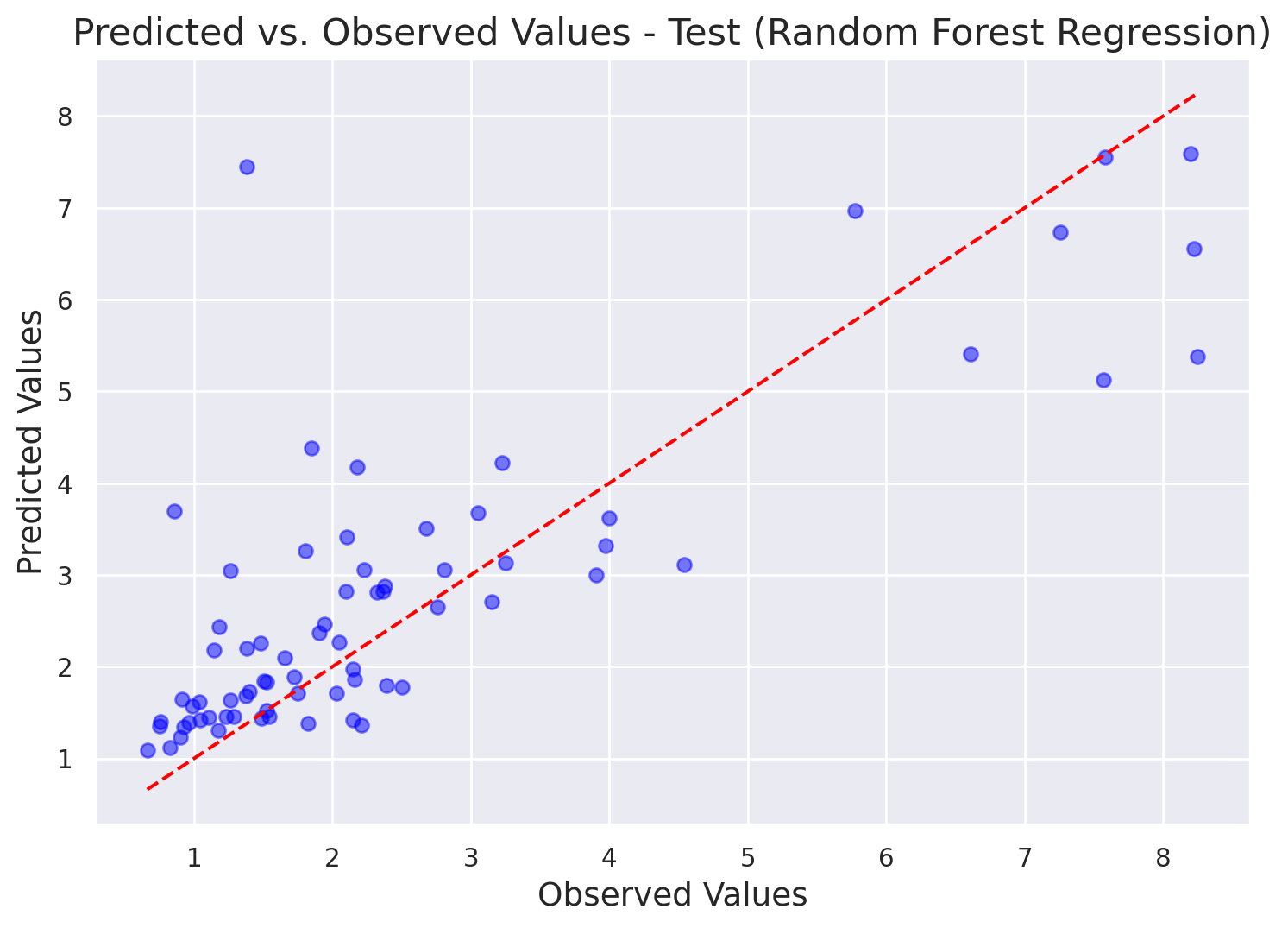

5. Calculate SHAP values

SHAP (SHapely Additive exPlanations) is a method that originally comes from cooperative game theory, where it was used to determine each player’s contribution on the resulting game score. Similarly, in machine learning, it is used to quantify the contribution of each covariate on the prediction target in an additive, linear manner (meaning that the contributions of features are summed). The SHAP are used to reveal if the contribution is positive or negative, and to quantify it. The values are in the units of the prediction target (in our case, mg/L), which makes them easy to interpret. Read more about SHAP in Molnar 2025 and https://shap.readthedocs.io/en/latest/.

The SHAP value method is model-agnostic, meaning that it can be used on various machine learning algorithms. For our Random Forest models, we will use the TreeSHAP (function TreeExplainer), which is a variant of SHAP made specifically for decision tree models. SHAP values are computationally quite expensive and might take long time if you have millions of data points.

# Calculate SHAP values
explainer = shap.TreeExplainer(regressor)
shap_values = explainer.shap_values(X_train)

Shap values are organised in an array of arrays by sample and then by the covariate.

shap_values

array([[-5.36666271e-03, -1.88318222e-02, -1.34617665e-02, ...,
        -1.22863556e-03, -1.28882906e-01, -1.59744522e-02],
       [ 1.88903182e-01, -2.85382651e-02, -9.85669941e-03, ...,
         1.49344477e-02,  1.72678670e-01,  2.10884832e-02],
       [-8.24545981e-02, -2.09307261e-02,  4.98129418e-03, ...,
         1.98363109e-03, -1.92131692e-01, -1.50710452e-02],
       ...,
       [-5.45506803e-02,  2.06487127e-02, -9.72199513e-03, ...,
         1.31034133e-02, -1.28973225e-01, -3.33952576e-02],
       [-8.82154124e-01, -4.94812332e-02, -6.20282270e-04, ...,
        -8.24274818e-02,  7.77009380e-02, -1.90850789e-02],
       [-4.69086937e-01, -3.44459380e-02,  2.59288673e-03, ...,
         1.74268347e-01,  9.27250026e-02,  6.54904839e-04]],
      shape=(167, 82))

The SHAP values can be calculated both globally (for the whole dataset) and locally (distinguishing individual instances). First, let’s plot SHAP globally using the summary plot.

This plot shows the absolute contribution of each feature. The features are ordered based on their importance, and here, 20 out of 82 most important features are plotted. On average, the highest contribution to the total nitrogen value is by the proportion of arable land in catchment (arable_prop), features mean rock content of the first layer (rock1_mean), silt % of the first soil layer (silt1_mean) and rip_veg_nat_prop (total area of riparian vegetation buffer around natural streams divided by catchment area), all exceeding 0.1 mg/L. All other features contributed by 0.1 mg/L or less.

NB! While SHAP might seem similar to permutation based feature importance, the latter describes feature contribution to the prediction accuracy, not to the target value! Please be mindful when interpreting the results.

The average impact of features on the prediction target, ordered by importance. The values are in units of the prediction target.

# SHAP summary bar plot

shap.summary_plot(shap_values=shap_values, features=X_train, feature_names=X_train.columns, plot_type="bar")
plt.tight_layout()

<Figure size 672x480 with 0 Axes>

For a more thorough exploration, it is always advisable to plot the summary beeswarm plot, where individual instances can be observed. The interpretation of the summary beeswarm plot is as follows: each point is the SHAP value in a distinct sampling location. Each feature has as many points as sampling locations in our dataset. The colour describes the covariate value relative to the range of covariate values in the dataset for each covariate separately. The red dots represent high values (for example, high rock content in the first layer), while blue represents low values.

The impact on the target value (in our case, total nitrogen mg/L) can be read from the x-axis: the more a certain point is positioned to the right, the higher the contribution, and vice versa; for example, high arable proportion in the catchment (arable_prop) results in up to 2 mg/L higher total nitrogen concentration in certain locations.

Besides that, we can see that features like rock content in the first layer (rock1_mean) and the arable proportion in the catchment (arable_prop) contribute positively to the target, since higher feature values result in higher contribution, while features like k1_mean (mean hydraulic conductivity of the first layer) and rip_veg_nat_prop (total area of riparian vegetation buffer around natural streams divided by catchment area) have a negative influence: lower values result in higher total nitrogen concentration.

As you can see, the feature’s contribution of high vs. low values is not symmetric. For example, low values of rip_veg_nat_prop contribute up to 2.6 mg/L increase on the target, while high values of the same feature decrease the total nitrogen content by only 0.6 mg/L at most.

SHAP values and partial dependence plots (below) are great tools for model validation: the model can see if the relationships revealed by the model are logical and correspond to the domain knowledge.

# SHAP summary beeswarm plot

plt.figure(figsize=(10, 24))
shap.summary_plot(shap_values=shap_values, features=X_train, feature_names=X_train.columns)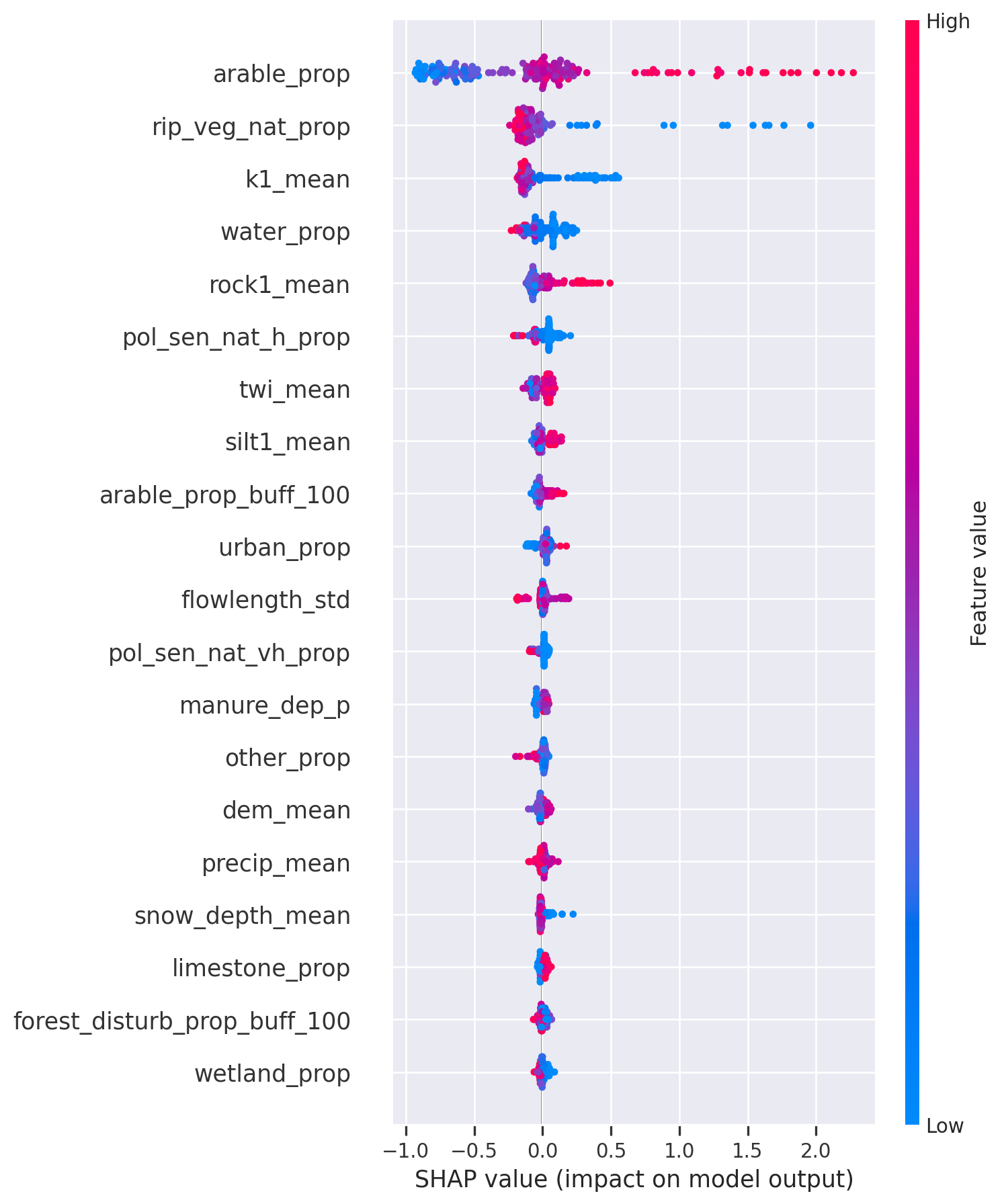

Explanation of some of the features

arable_prop - the proportion of arable land in the catchment

rip_veg_nat_prop - total area of riparian vegetation buffer around natural streams divided by catchment area

k1_mean - mean hydraulic conductivity of the first layer

rock1_mean - rock content in the first soil layer

water_prop - proportion f waterbodies in the catchment

twi_mean - mean topographic wetness index

silt1_mean - mean silt percentage in soil first layer

manure_dep_p - manure deposition

To better understand how each predictor contributes to the model and how it is related to the target variable, we can use partial dependence plots. We don’t want to plot all 82 features, and therefore, we will subset the 10 most important covariates based on SHAP values.

In addition, we also want to perform some feature reduction.

Feature reduction is important because:

Item Feature reduction helps to reduce potential overfitting and improve its generalization ability.
Item Models with fewer features require less computational resources and time to train and also less preparation time and storage on the input data.
Item A smaller set of features can make it easier to understand how the model is making predictions.
Item Although Random Forest is quite good at dealing with redundancy; then it is still preferred to remove highly correlated features because they start diluting each other’s contribution.

5.1 Top 10 features with the highest SHAP value

Let’s extract top 10 features and keep only those in the model.

#extracting top 10 features based on SHAP values
feature_names = X_train.columns
rf_resultX = pd.DataFrame(shap_values, columns = feature_names)
vals = np.abs(rf_resultX.values).mean(0)
shap_importance = pd.DataFrame(list(zip(feature_names, vals)),
                                  columns=["feature","feature_importance_vals"])
shap_importance.sort_values(by=["feature_importance_vals"],
                               ascending=False, inplace=True)
shap_importance[:10]

	feature	feature_importance_vals
0	arable_prop	0.521271
45	rip_veg_nat_prop	0.189679
32	k1_mean	0.165786
80	water_prop	0.094160
48	rock1_mean	0.081662
41	pol_sen_nat_h_prop	0.060887
77	twi_mean	0.051824
56	silt1_mean	0.043601
1	arable_prop_buff_100	0.040729
79	urban_prop	0.039152

5.2 Plot the partial dependence

Partial Dependence plots show the marginal effect of a feature on a target in a ML model, that is, the contribution of a specific feature on the target after the average impacts of other features have been removed. Usually, partial dependence plots are drawn for one to two features at the time as the interpretation of more features becomes increasingly complex.

With these plots, one can determine if the influence of the feature on the prediction target is linear or non-linear. Moreover, the x-axis shows the values of the respective feature, while the y-axis visualises the target values (in our case, total nitrogen, mg/L). Thus, these plots are intuitive to understand and interpret and certain thresholds of influence can be determined.

For example, with an increasing proportion of arable land (feature “arable_prop”), the concentration of total nitrogen increases. A steep increase is noted when the arable proportion exceeds 40%, rising from around 2.5 mg/L to around 4.5 mg/L. As with SHAP, these plots are a great validation tool. New insights can also be gained, however caution should be exercised when interpreting the relationships. For example, keep in mind that the marks of data (small black vertical lines on the x-axis) indicate value density around certain values in your dataset, therefore a lower certainty is in the data range with low number of points (e.g., range 20-40 vs. range 60-80 for the feature k1_mean).

# Create partial dependence plot (Full Model)
fig, ax = plt.subplots(figsize=(12, 12))
disp = PartialDependenceDisplay.from_estimator(regressor, X_train, shap_importance[:10]["feature"].values, ax=ax)
fig.subplots_adjust(hspace=0.3)
fig.tight_layout()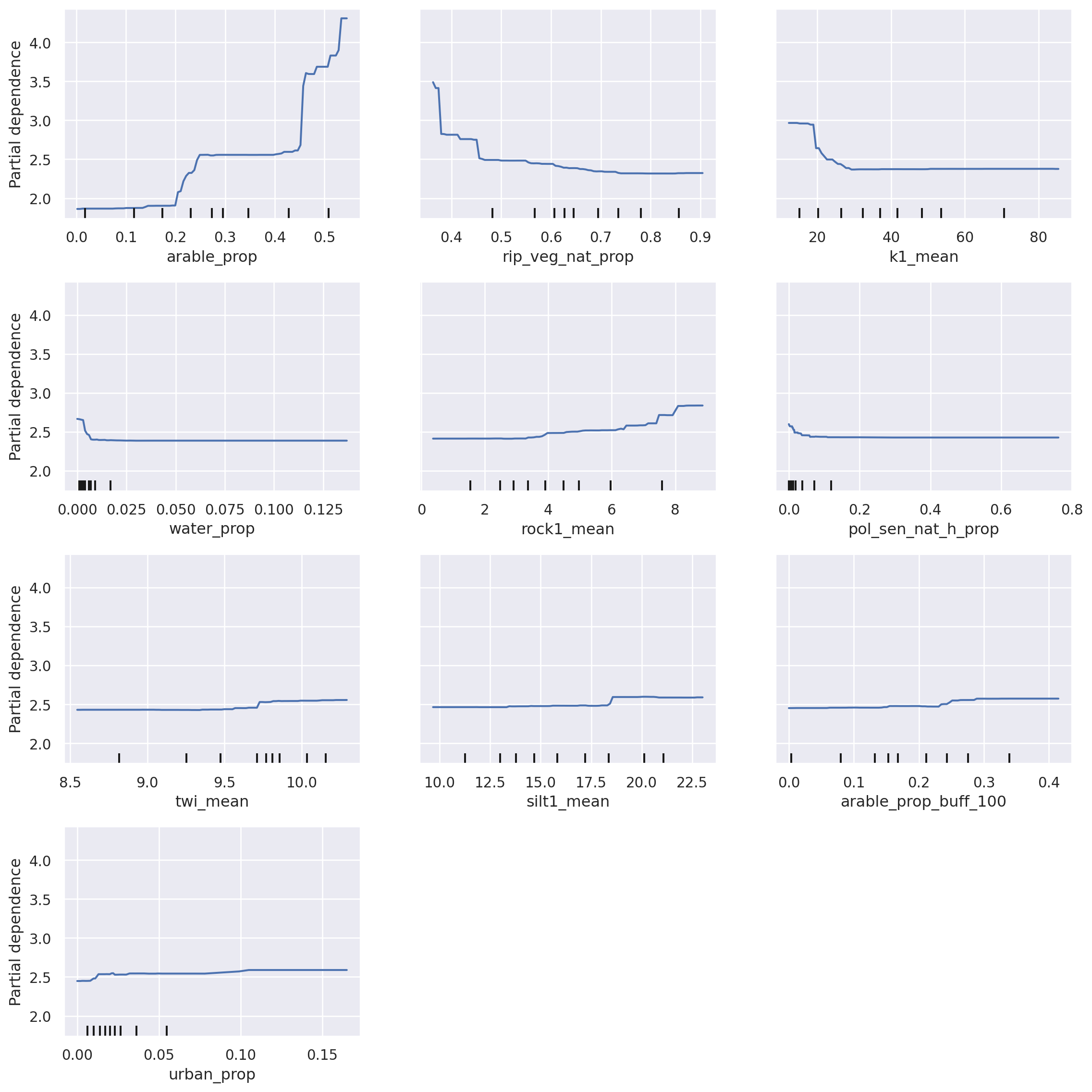

6. Reduce the number of features in the model based on SHAP values

As a general rule, we are interested in models needing as little features as possible due to computational etc. limitations. There are various feature reduction methods, such as permutation based feature importance, forward feature selection, and others. Now we will decrease our feature set using the results of SHAP and will explore the difference in the prediction accuracy.

We will use the 10 most influential features (from the original 82) as determined by SHAP and will re-train the Random Forest model with this decreased feature set.

abs_mean_shap_df = shap_importance[:10]

# List of most important features
n_features = 10
top_features = abs_mean_shap_df["feature"].head(n_features).to_list()
print(top_features)

['arable_prop', 'rip_veg_nat_prop', 'k1_mean', 'water_prop', 'rock1_mean', 'pol_sen_nat_h_prop', 'twi_mean', 'silt1_mean', 'arable_prop_buff_100', 'urban_prop']

We subset the relevant features from the original training dataset.

# Generate new training and test feature sets
X_train_reduced = X_train[top_features]
X_test_reduced = X_test[top_features]
X_train_reduced

	arable_prop	rip_veg_nat_prop	k1_mean	water_prop	rock1_mean	pol_sen_nat_h_prop	twi_mean	silt1_mean	arable_prop_buff_100	urban_prop
29	0.351	0.670	54.825	0.009	3.015	0.120	9.081	11.058	0.170	0.030
124	0.448	0.653	13.490	0.002	5.806	0.002	10.148	24.763	0.222	0.023
75	0.348	0.709	27.407	0.051	6.353	0.296	7.579	16.814	0.231	0.034
82	0.215	0.801	10.666	0.001	4.250	0.013	9.923	24.458	0.159	0.012
5	0.089	0.690	36.952	0.005	1.638	0.007	9.941	22.782	0.114	0.008
...	...	...	...	...	...	...	...	...	...	...
106	0.012	0.901	31.204	0.005	0.341	0.000	9.331	17.253	0.016	0.032
14	0.316	0.615	38.923	0.005	7.612	0.025	9.605	17.265	0.163	0.021
92	0.295	0.498	22.929	0.007	3.297	0.013	9.651	20.454	0.282	0.050
179	0.042	0.837	72.675	0.001	2.551	0.000	9.795	11.674	0.106	0.003
102	0.017	0.837	35.879	0.002	0.069	0.000	9.332	15.812	0.057	0.136

167 rows × 10 columns

6.1 Train model on reduced data

Again, we will determine the optimal hyperparameters with the exact same methodology as before, but on the reduced training set.

%%time

# Perform search for hyperparameters
params_reduced = search_hyperparams(X_train_reduced, y_train, random_state)
params_reduced

Fitting 5 folds for each of 28 candidates, totalling 140 fits

/usr/lib64/python3.13/site-packages/sklearn/model_selection/_search.py:317: UserWarning: The total space of parameters 28 is smaller than n_iter=100. Running 28 iterations. For exhaustive searches, use GridSearchCV.
  warnings.warn(

CPU times: user 385 ms, sys: 29.4 ms, total: 415 ms
Wall time: 2.66 s

{'n_estimators': np.int64(50), 'max_depth': np.int64(20), 'oob_score': True}

Let’s train the model with the optimal hyperparameters and the reduced training set the same way we did before.

# RF regressor
regressor_reduced = RandomForestRegressor()

# Set hyperparameters
regressor_reduced.set_params(**params_reduced)

# Fit model
regressor_reduced.fit(X_train_reduced, y_train)

RandomForestRegressor(max_depth=np.int64(20), n_estimators=np.int64(50),
                      oob_score=True)

# Calculate accuracy on training set
r2_train_reduced = regressor_reduced.score(X_train_reduced, y_train)
print(f"R-squared train score: {r2_train_reduced:.2f}")

R-squared train score: 0.93

As you can see, the accuracy on the training and test set with the lower feature set has remained practically the same or even improved with less data needed. Great! Keep in mind though, that this is not a guarantee- the scores can decrease, depending on the data, etc.

# Calculate OOB R2
oob_r2 = regressor_reduced.oob_score_
print(f"OOB reduced R-squared score: {oob_r2:.2f}")

OOB reduced R-squared score: 0.56

# Predict
Y_train_pred_reduced = regressor_reduced.predict(X_train_reduced)
Y_test_pred_reduced = regressor_reduced.predict(X_test_reduced)

# Calculate accuracy on test set
r2_test_reduced = r2_score(y_test, Y_test_pred_reduced)
print(f"R-squared test score: {r2_test_reduced:.2f}")

R-squared test score: 0.62

7. SHAP analysis of the new model

Now, we will again plot the SHAP values and explore the differences in contribution between the full and the decrease data sets.

# Calculate SHAP values
explainer_reduced = shap.TreeExplainer(regressor_reduced)
shap_values_reduced = shap.TreeExplainer(regressor_reduced).shap_values(X_train_reduced)

# SHAP summary beeswarm plot
shap.summary_plot(shap_values=shap_values_reduced, features=X_train_reduced, feature_names=X_train_reduced.columns)
plt.tight_layout()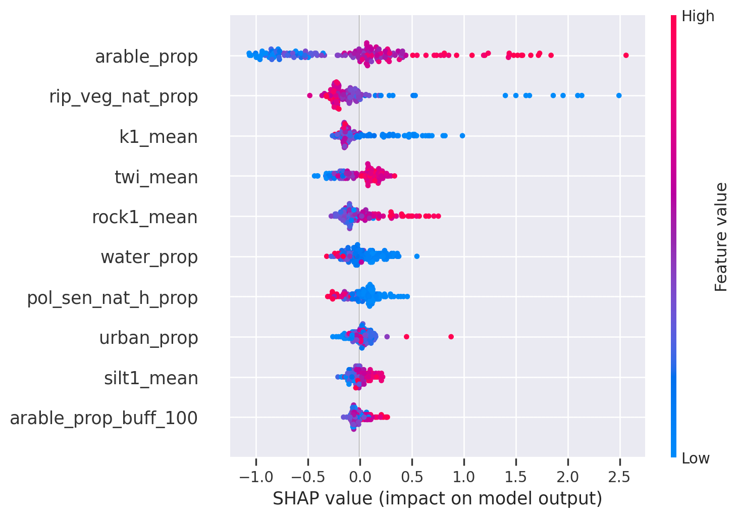

<Figure size 672x480 with 0 Axes>

The order has remained the same but the influence has increased a bit. That is a good indicator, showing that the model is quite robust and you have meaningful predictors.

Let’s look at the partial dependence plots once again. As before, the relationships remain the same. As with SHAP, these plots are a great validation tool. New insights can also be gained, however caution should be exercised when interpreting the relationships.

# Create partial dependence plot
fig, ax = plt.subplots(figsize=(12, 12))
disp = PartialDependenceDisplay.from_estimator(regressor_reduced, X_train_reduced, X_train_reduced.columns, ax=ax)
fig.subplots_adjust(hspace=0.3)
fig.tight_layout()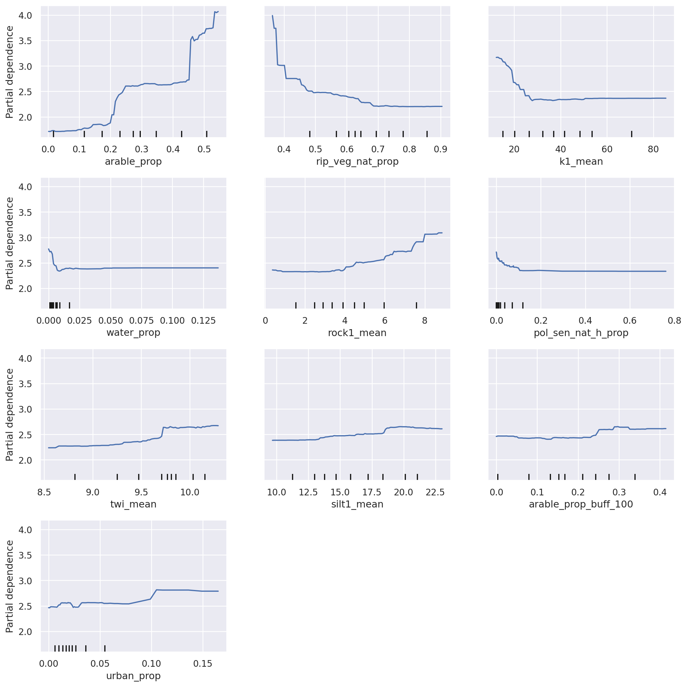

8. Add coordinates as covariates

Machine learning is not inherently spatial; however, often enough, it will indirectly already learn/capture the spatial relationships. For many phenomena, spatial relationships are relevant (Toblern’s first law) and therefore, incorporating spatial aspects into machine learning can be useful. There are many ways in which spatial aspects can be incorporated into machine learning. In this lesson, we will look into the simplest method - using coordinates (X and Y as covariates). If you want to know more about spatial ML then see Jemeljanova et al. 2024 and Kmoch et al. 2025

In machine learning, incorporating coordinate data can encode relevant information about location, proximity, and spatial relationships between data points. By explicitly including this spatial context as features, machine learning models can learn patterns and dependencies that might be entirely missed when relying solely on non-spatial attributes. This can significantly improve predictive accuracy for tasks ranging from geographic forecasting and resource allocation to understanding environmental patterns. However, one also has to be careful because spatial autocorrelation can create overly optimistic predictions (Ploton et al. 2020).

Let’s add coordinates as covariates to our model. Out feature dataframe X_train_reduced does not have geometry data anymore. The geometry data is in the original dataframe obs_data. Therefore, we need to extract the coordinates from the original dataframe and join them back in to the X_train_reduced

#Check the X_train_reduced
X_train_reduced

	arable_prop	rip_veg_nat_prop	k1_mean	water_prop	rock1_mean	pol_sen_nat_h_prop	twi_mean	silt1_mean	arable_prop_buff_100	urban_prop
29	0.351	0.670	54.825	0.009	3.015	0.120	9.081	11.058	0.170	0.030
124	0.448	0.653	13.490	0.002	5.806	0.002	10.148	24.763	0.222	0.023
75	0.348	0.709	27.407	0.051	6.353	0.296	7.579	16.814	0.231	0.034
82	0.215	0.801	10.666	0.001	4.250	0.013	9.923	24.458	0.159	0.012
5	0.089	0.690	36.952	0.005	1.638	0.007	9.941	22.782	0.114	0.008
...	...	...	...	...	...	...	...	...	...	...
106	0.012	0.901	31.204	0.005	0.341	0.000	9.331	17.253	0.016	0.032
14	0.316	0.615	38.923	0.005	7.612	0.025	9.605	17.265	0.163	0.021
92	0.295	0.498	22.929	0.007	3.297	0.013	9.651	20.454	0.282	0.050
179	0.042	0.837	72.675	0.001	2.551	0.000	9.795	11.674	0.106	0.003
102	0.017	0.837	35.879	0.002	0.069	0.000	9.332	15.812	0.057	0.136

167 rows × 10 columns

#Check the obs_data
obs_data

	site_code	obs_id	obs_value	arable_prop	arable_prop_buff_100	arable_prop_buff_1000	arable_prop_buff_500	area	awc1_min	awc1_max	...	tri_mean	tri_std	twi_min	twi_max	twi_mean	twi_std	urban_prop	water_prop	wetland_prop	geometry
0	SJA8127000	161	1.0288	0.086	0.175	0.092	0.124	1.512569e+08	0.178	0.212	...	0.119	0.176	2.206	14.725	9.732	1.706	0.006	0.005	0.129	POINT (696315 6546937)
1	SJA9900000	200	1.3402	0.182	0.170	0.178	0.190	8.071414e+08	0.173	0.215	...	0.100	0.191	1.725	15.356	9.827	1.375	0.026	0.008	0.087	POINT (669868 6591973)
2	SJA3956000	90	6.6156	0.536	0.340	0.520	0.464	4.229881e+08	0.169	0.207	...	0.112	0.150	1.869	15.563	9.910	1.513	0.049	0.003	0.006	POINT (636008 6603086)
3	SJA1934000	40	1.6676	0.243	0.134	0.172	0.156	2.132077e+08	0.173	0.211	...	0.109	0.183	1.842	14.976	9.745	1.348	0.056	0.004	0.014	POINT (700294 6592517)
4	SJA7837000	157	2.8696	0.293	0.321	0.330	0.352	3.100426e+08	0.173	0.208	...	0.111	0.151	1.859	15.576	9.724	1.397	0.111	0.007	0.058	POINT (520653 6588232)
...	...	...	...	...	...	...	...	...	...	...	...	...	...	...	...	...	...	...	...	...	...
234	SJB3503000	238	8.2250	0.537	0.316	0.523	0.453	1.122941e+08	0.174	0.205	...	0.099	0.111	2.279	15.563	10.033	1.392	0.028	0.002	0.014	POINT (633230 6585334)
235	SJA3731000	84	1.7250	0.200	0.065	0.122	0.085	6.085978e+07	0.175	0.206	...	0.124	0.223	1.842	14.565	9.663	1.395	0.072	0.003	0.009	POINT (698754 6586118)
236	SJA0813000	17	3.2500	0.452	0.223	0.499	0.475	4.023375e+07	0.174	0.207	...	0.207	0.272	2.373	16.631	9.019	2.097	0.033	0.007	0.014	POINT (619933 6581023)
237	SJA8884000	175	3.3000	0.242	0.176	0.232	0.225	1.930663e+09	0.164	0.218	...	0.105	0.145	1.464	15.329	9.728	1.468	0.025	0.010	0.106	POINT (551221 6591443)
238	SJA1953000	41	3.0050	0.479	0.266	0.498	0.455	9.860328e+07	0.172	0.207	...	0.178	0.246	2.294	16.631	9.266	1.959	0.028	0.004	0.027	POINT (619319 6581605)

239 rows × 86 columns

# Extract X coordinates from the geometry column from the original dataframe
obs_data['X'] = obs_data['geometry'].x

# Extract Y coordinates from the geometry column from the original dataframe
obs_data['Y'] = obs_data['geometry'].y

obs_data.head()

	site_code	obs_id	obs_value	arable_prop	arable_prop_buff_100	arable_prop_buff_1000	arable_prop_buff_500	area	awc1_min	awc1_max	...	twi_min	twi_max	twi_mean	twi_std	urban_prop	water_prop	wetland_prop	geometry	X	Y
0	SJA8127000	161	1.0288	0.086	0.175	0.092	0.124	151256900.0	0.178	0.212	...	2.206	14.725	9.732	1.706	0.006	0.005	0.129	POINT (696315 6546937)	696315.0	6546937.0
1	SJA9900000	200	1.3402	0.182	0.170	0.178	0.190	807141375.0	0.173	0.215	...	1.725	15.356	9.827	1.375	0.026	0.008	0.087	POINT (669868 6591973)	669868.0	6591973.0
2	SJA3956000	90	6.6156	0.536	0.340	0.520	0.464	422988125.0	0.169	0.207	...	1.869	15.563	9.910	1.513	0.049	0.003	0.006	POINT (636008 6603086)	636008.0	6603086.0
3	SJA1934000	40	1.6676	0.243	0.134	0.172	0.156	213207725.0	0.173	0.211	...	1.842	14.976	9.745	1.348	0.056	0.004	0.014	POINT (700294 6592517)	700294.0	6592517.0
4	SJA7837000	157	2.8696	0.293	0.321	0.330	0.352	310042550.0	0.173	0.208	...	1.859	15.576	9.724	1.397	0.111	0.007	0.058	POINT (520653 6588232)	520653.0	6588232.0

5 rows × 88 columns

# Join the coordinates from the original dataframe to the reduced training set
X_train_reduced_with_coords = X_train_reduced.join(obs_data[['X', 'Y']], how='left')
X_train_reduced_with_coords.head()

	arable_prop	rip_veg_nat_prop	k1_mean	water_prop	rock1_mean	pol_sen_nat_h_prop	twi_mean	silt1_mean	arable_prop_buff_100	urban_prop	X	Y
29	0.351	0.670	54.825	0.009	3.015	0.120	9.081	11.058	0.170	0.030	683677.0	6462977.0
124	0.448	0.653	13.490	0.002	5.806	0.002	10.148	24.763	0.222	0.023	592142.0	6527965.0
75	0.348	0.709	27.407	0.051	6.353	0.296	7.579	16.814	0.231	0.034	650343.0	6421214.0
82	0.215	0.801	10.666	0.001	4.250	0.013	9.923	24.458	0.159	0.012	628757.0	6496513.0
5	0.089	0.690	36.952	0.005	1.638	0.007	9.941	22.782	0.114	0.008	682346.0	6543218.0

# Join the coordinates from the original dataframe to the reduced test set
X_test_reduced_with_coords = X_test_reduced.join(obs_data[['X', 'Y']], how='left')
X_test_reduced_with_coords.head()

	arable_prop	rip_veg_nat_prop	k1_mean	water_prop	rock1_mean	pol_sen_nat_h_prop	twi_mean	silt1_mean	arable_prop_buff_100	urban_prop	X	Y
24	0.344	0.679	39.615	0.012	3.065	0.128	8.334	13.369	0.195	0.033	660864.0	6462472.0
6	0.241	0.678	35.526	0.010	4.547	0.020	9.724	16.974	0.174	0.026	548527.0	6591802.0
93	0.461	0.562	16.573	0.001	5.971	0.007	10.210	24.178	0.318	0.023	593325.0	6530980.0
109	0.000	0.247	5.837	0.034	0.161	0.000	10.032	24.267	0.000	0.000	498224.0	6484291.0
104	0.271	0.699	39.381	0.003	2.844	0.000	9.730	17.398	0.215	0.015	488342.0	6524192.0

# Perform a search for hyperparameters
params_reduced_coord = search_hyperparams(X_train_reduced_with_coords, y_train, random_state)
params_reduced_coord

/usr/lib64/python3.13/site-packages/sklearn/model_selection/_search.py:317: UserWarning: The total space of parameters 28 is smaller than n_iter=100. Running 28 iterations. For exhaustive searches, use GridSearchCV.
  warnings.warn(

Fitting 5 folds for each of 28 candidates, totalling 140 fits

{'n_estimators': np.int64(175), 'max_depth': np.int64(20), 'oob_score': True}

Let’s train the new model with spatial covariates (X and Y)

# RF regressor
regressor_reduced_coords = RandomForestRegressor()

# Set hyperparameters
regressor_reduced_coords.set_params(**params_reduced)

# Fit model
regressor_reduced_coords.fit(X_train_reduced_with_coords, y_train)

RandomForestRegressor(max_depth=np.int64(20), n_estimators=np.int64(50),
                      oob_score=True)

# Calculate accuracy on training set
r2_train_reduced_coords = regressor_reduced_coords.score(X_train_reduced_with_coords, y_train)
print(f"R-squared train score: {r2_train_reduced_coords:.2f}")

R-squared train score: 0.94

# Calculate OOB R2
oob_r2 = regressor_reduced_coords.oob_score_
print(f"OOB reduced R-squared score: {oob_r2:.2f}")

OOB reduced R-squared score: 0.59

The spatial covariates did not significantly improve the model but also did not make it worse. To better understand how they contribute, we need to look at SHAP values again.

# Predict
Y_train_pred_reduced_coords = regressor_reduced_coords.predict(X_train_reduced_with_coords)
Y_test_pred_reduced_coords = regressor_reduced_coords.predict(X_test_reduced_with_coords)

# Calculate accuracy on test set
r2_test_reduced_coords = r2_score(y_test, Y_test_pred_reduced_coords)
print(f"R-squared test score: {r2_test_reduced:.2f}")

R-squared test score: 0.62

# Calculate SHAP values
explainer_reduced_coords = shap.TreeExplainer(regressor_reduced_coords)
shap_values_reduced_coords = shap.TreeExplainer(regressor_reduced_coords).shap_values(X_train_reduced_with_coords)

# SHAP summary beeswarm plot
shap.summary_plot(shap_values=shap_values_reduced_coords, features=X_train_reduced_with_coords, feature_names=X_train_reduced_with_coords.columns)
plt.tight_layout()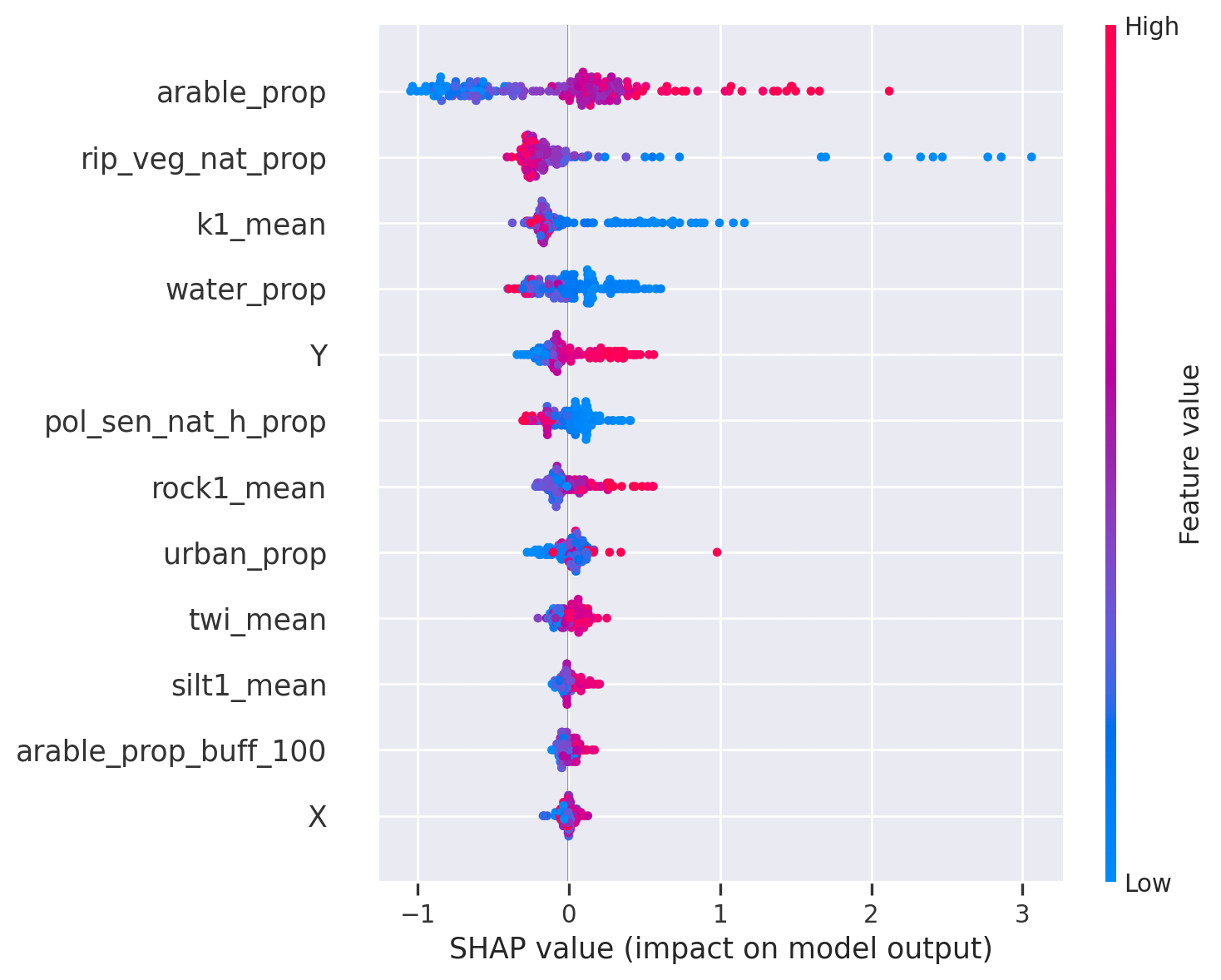

<Figure size 672x480 with 0 Axes>

As you can see, that the main predictors (arable_prop, rip_veg_nat_prop, k1_mean) did not change but Y has popped up as a covariate and rock1_mean has moved downwards. There is a positive relationship between Y and total nitrogen, indicating that more north is higher total nitrogen. There can be several explanations but in general there are more polluted rivers in northern Estonia because of human population and industry. As we don’t have humap population and industry as covariates then Y is indirectly capturing that pattern. That tends to happen quite often that spatial covariates can be sort of replacement for covariates that we don’t have in our data.

9. Plot the predictions spatially

Now, we will plot all predictions spatially (for both train and test locations) of our target value (total nitrogen, mg/L) from our model with the reduced and spatial feature set. First, we will create a dataframe with all locations.

# Concatenate reduced features and sort by index
X_reduced_coords = pd.concat([X_train_reduced_with_coords, X_test_reduced_with_coords]).sort_index()
X_reduced_coords.head()

	arable_prop	rip_veg_nat_prop	k1_mean	water_prop	rock1_mean	pol_sen_nat_h_prop	twi_mean	silt1_mean	arable_prop_buff_100	urban_prop	X	Y
0	0.086	0.640	57.067	0.005	0.117	0.007	9.732	12.941	0.175	0.006	696315.0	6546937.0
1	0.182	0.606	41.811	0.008	4.713	0.016	9.827	18.374	0.170	0.026	669868.0	6591973.0
2	0.536	0.402	26.810	0.003	8.828	0.042	9.910	19.020	0.340	0.049	636008.0	6603086.0
3	0.243	0.679	52.092	0.004	4.079	0.034	9.745	14.901	0.134	0.056	700294.0	6592517.0
4	0.293	0.580	40.121	0.007	6.022	0.009	9.724	16.916	0.321	0.111	520653.0	6588232.0

Next, we will use our trained model to predict the target values for all locations.

# Predict with the reduced model
predictions = regressor_reduced_coords.predict(X_reduced_coords)
display(predictions)

array([1.181444  , 1.483134  , 5.95048533, 2.128146  , 2.73988467,
       1.064322  , 2.913492  , 3.167748  , 2.555716  , 2.737552  ,
       1.242678  , 1.478302  , 1.9619    , 4.22823   , 3.39292   ,
       2.359296  , 1.084972  , 7.11845133, 1.258124  , 1.70578   ,
       2.38670667, 6.53121333, 1.5237    , 2.074596  , 1.447572  ,
       1.202454  , 1.025296  , 1.152088  , 1.390652  , 1.503872  ,
       1.715196  , 1.590852  , 2.648064  , 2.99552867, 5.18156933,
       2.960472  , 3.121522  , 4.86019067, 2.837144  , 1.277688  ,
       9.69387333, 4.56488933, 4.215252  , 3.452646  , 3.142172  ,
       1.310042  , 5.070452  , 1.584912  , 1.115389  , 1.329764  ,
       1.525048  , 2.614614  , 1.81132   , 1.695755  , 1.268245  ,
       2.18427733, 1.539824  , 2.91385   , 3.052012  , 3.37502667,
       3.53017467, 1.989154  , 1.82627   , 1.400924  , 7.96210667,
       8.15483333, 8.13107333, 4.984238  , 1.273952  , 2.273786  ,
       2.396676  , 0.986664  , 1.092892  , 1.16852   , 2.341696  ,
       0.886788  , 0.971944  , 1.811364  , 2.03036   , 5.43048267,
       2.90130533, 3.888388  , 2.789016  , 2.98893067, 3.03010933,
       3.96287933, 2.55213867, 1.63254   , 1.827055  , 3.236332  ,
       1.273051  , 2.06716   , 1.99756   , 4.28220933, 2.710396  ,
       3.738366  , 1.310042  , 3.22061333, 3.66550733, 2.30606667,
       1.840976  , 1.365165  , 3.439428  , 3.31559467, 3.06932533,
       1.456094  , 1.86926   , 1.378296  , 1.387862  , 4.15217067,
       2.076589  , 1.52852   , 1.76597   , 1.789924  , 1.632338  ,
       1.480862  , 1.32446   , 1.997064  , 1.660628  , 1.278664  ,
       1.452516  , 1.39004   , 1.582544  , 1.424904  , 3.662996  ,
       3.64436933, 8.04238533, 3.05020533, 2.541052  , 2.404116  ,
       1.347196  , 2.475164  , 1.187882  , 1.247459  , 1.00368   ,
       2.14566933, 1.388432  , 1.288953  , 1.00552   , 0.951432  ,
       0.977424  , 1.077482  , 1.034065  , 0.989392  , 1.13471   ,
       1.00152   , 1.084654  , 1.163814  , 0.90394   , 1.60775   ,
       1.426296  , 1.98904467, 2.47008533, 1.46654   , 1.046509  ,
       1.22129   , 0.86003   , 0.994092  , 0.904656  , 1.96220467,
       0.984496  , 2.62279867, 1.222936  , 1.031324  , 4.333958  ,
       2.94776467, 1.897148  , 1.949274  , 2.1457    , 1.595012  ,
       1.24016   , 1.78276467, 2.839134  , 2.24485067, 2.369284  ,
       2.432744  , 4.25676067, 2.184736  , 4.28252133, 1.20035   ,
       3.76733   , 2.867533  , 2.359738  , 1.198502  , 2.431044  ,
       1.93095867, 1.741647  , 1.00142   , 0.956624  , 1.06616   ,
       2.14545333, 2.368456  , 2.587019  , 1.867948  , 1.912986  ,
       2.270662  , 2.597084  , 4.920276  , 3.342882  , 2.88036   ,
       2.213634  , 2.62375   , 1.139798  , 3.190186  , 7.52291533,
       8.03759467, 1.731174  , 2.158928  , 1.892478  , 6.49434467,
       3.099488  , 1.362744  , 1.525224  , 7.09298933, 3.504272  ,
       3.509618  , 2.595824  , 2.07694   , 5.28327533, 8.13551067,
       4.32616267, 3.406804  , 5.58552733, 6.39989467, 3.733764  ,
       1.424094  , 1.587487  , 5.59167   , 3.037848  , 2.29523333,
       1.898802  , 7.438904  , 2.713512  , 2.167118  , 7.30547333,
       1.800744  , 4.2694    , 3.0659    , 3.804504  ])

# Add predictions to observation data
obs_data_pred = obs_data.copy()
obs_data_pred["pred_value"] = predictions
obs_data_pred.head()

	site_code	obs_id	obs_value	arable_prop	arable_prop_buff_100	arable_prop_buff_1000	arable_prop_buff_500	area	awc1_min	awc1_max	...	twi_max	twi_mean	twi_std	urban_prop	water_prop	wetland_prop	geometry	X	Y	pred_value
0	SJA8127000	161	1.0288	0.086	0.175	0.092	0.124	151256900.0	0.178	0.212	...	14.725	9.732	1.706	0.006	0.005	0.129	POINT (696315 6546937)	696315.0	6546937.0	1.181444
1	SJA9900000	200	1.3402	0.182	0.170	0.178	0.190	807141375.0	0.173	0.215	...	15.356	9.827	1.375	0.026	0.008	0.087	POINT (669868 6591973)	669868.0	6591973.0	1.483134
2	SJA3956000	90	6.6156	0.536	0.340	0.520	0.464	422988125.0	0.169	0.207	...	15.563	9.910	1.513	0.049	0.003	0.006	POINT (636008 6603086)	636008.0	6603086.0	5.950485
3	SJA1934000	40	1.6676	0.243	0.134	0.172	0.156	213207725.0	0.173	0.211	...	14.976	9.745	1.348	0.056	0.004	0.014	POINT (700294 6592517)	700294.0	6592517.0	2.128146
4	SJA7837000	157	2.8696	0.293	0.321	0.330	0.352	310042550.0	0.173	0.208	...	15.576	9.724	1.397	0.111	0.007	0.058	POINT (520653 6588232)	520653.0	6588232.0	2.739885

5 rows × 89 columns

Now, we will plot our predicted values.

# Create interactive plot of predicted values
obs_data_pred.explore(
    column="pred_value",
    cmap="YlOrRd",
    tooltip=["site_code", "obs_value", "pred_value"],
    marker_kwds={"radius": 4},
    style_kwds={"color": "black", "weight": 1, "fillOpacity": 0.9}
)

Make this Notebook Trusted to load map: File -> Trust Notebook

Residuals are the difference between the observed and predicted values. If residuals are spatially autocorrelated (meaning that values in close vicinity are similar), it indicates that there might be a feature missing. This information can be used to further improve the model.

# Calculate residuals between observed and predicted values
obs_data_pred["residual"] = obs_data_pred["obs_value"] - obs_data_pred["pred_value"]

# Create interactive plot of residuals
obs_data_pred.explore(
    column="residual",
    cmap="RdBu_r",
    tooltip=["site_code", "obs_value", "pred_value", "residual"],
    marker_kwds={"radius": 4},
    style_kwds={"color": "black", "weight": 1, "fillOpacity": 0.9},
    vmin=-5,  # Set the minimum color value
    vmax=5   # Set the maximum color value
)

Make this Notebook Trusted to load map: File -> Trust Notebook

# Calculate residual percentage
obs_data_pred["residual_percentage"] = (obs_data_pred["residual"]/obs_data_pred["obs_value"])* 100

# Create interactive plot of residual percentage
obs_data_pred.explore(
    column="residual_percentage",
    cmap="RdBu_r",
    tooltip=["site_code", "obs_value", "pred_value", "residual", "residual_percentage"],
    marker_kwds={"radius": 4},
    style_kwds={"color": "black", "weight": 1, "fillOpacity": 0.9},
    vmin=-100,  # Set the minimum color value
    vmax=100   # Set the maximum color value
)

Make this Notebook Trusted to load map: File -> Trust Notebook

Next, let’s explore the observed and predicted values. The plot indicates that the model overestimated the some of the low values and underestimated some of the high values, which is characteristic of Random Forest models. It could be due to the characteristics of how data is subsampled for the decision trees, meaning that the extreme values are not always included in training each tree, therefore the model does not learn all the possible value combinations.

# Make predictions on the test set
y_predicted_reduced = regressor_reduced_coords.predict(X_test_reduced_with_coords)
y_observed = y_test


# Create the plot
plt.figure(figsize=(9, 6))
plt.scatter(y_observed, y_predicted_reduced, color='blue', alpha=0.5)

# Add a diagonal line for perfect predictions
min_val = min(np.min(y_observed), np.min(y_predicted_reduced))
max_val = max(np.max(y_observed), np.max(y_predicted_reduced))
plt.plot([min_val, max_val], [min_val, max_val], color='red', linestyle='--')

# Add labels and title
plt.xlabel("Observed Values", fontsize=14)
plt.ylabel("Predicted Values", fontsize=14)
plt.title("Predicted vs. Observed Values - Test (Random Forest Regression)", fontsize=16)

plt.grid(True)
plt.show()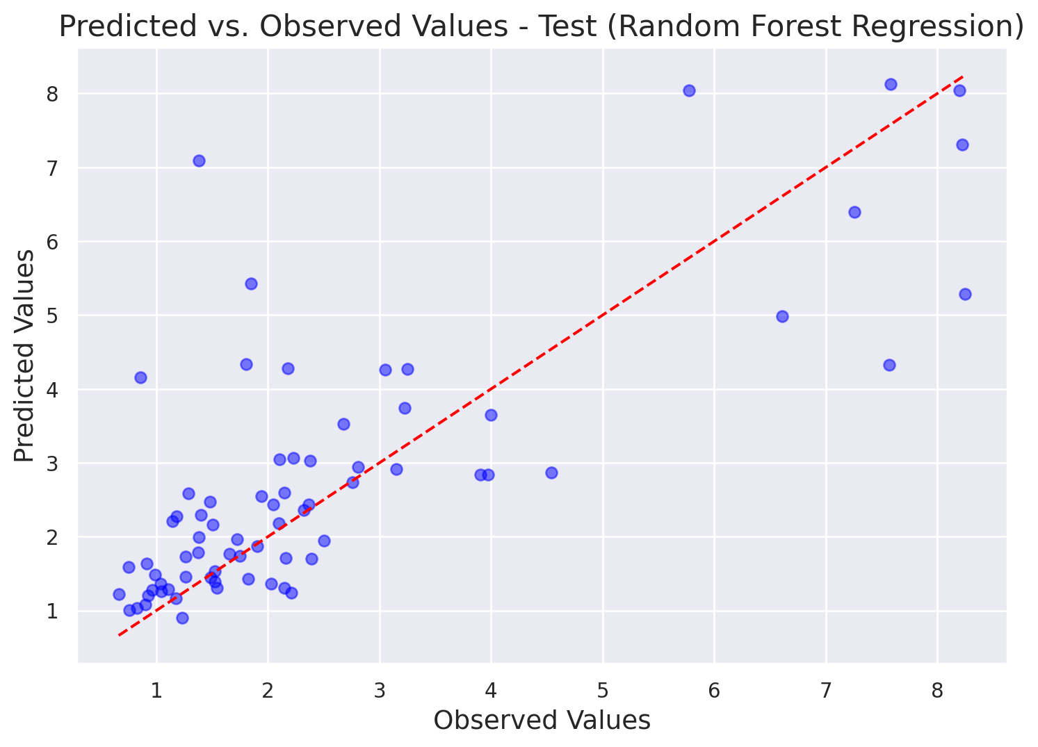

References

Bergstra, J., Bengio, Y., (2012). Random Search for Hyper-Parameter Optimization. Journal of Machine Learning Research, 13(10), 281–305. http://jmlr.org/papers/v13/bergstra12a.html

Breiman, L. Random Forests. Machine Learning 45, 5–32 (2001). https://doi-org.ezproxy.utlib.ut.ee/10.1023/A:1010933404324

Jemeljanova, Marta, Kmoch, Alexander, Uuemaa, Evelyn (2024). Adapting machine learning for environmental spatial data - A review. Ecological Informatics, 81, ARTN 102634. DOI: 10.1016/j.ecoinf.2024.102634.

Kmoch, Alexander, Harrison, Clay Taylor, Choi, Jeonghwan, Uuemaa, Evelyn (2025). Spatial autocorrelation in machine learning for modelling soil organic carbon. Ecological Informatics, 103057. DOI: 10.1016/j.ecoinf.2025.103057.

Molnar, C. (2025). Interpretable Machine Learning: A Guide for Making Black Box Models Explainable (3rd ed.). https://christophm.github.io/interpretable-ml-book/cite.html

Ploton, P., Mortier, F., Réjou-Méchain, M. et al. (2020). Spatial validation reveals poor predictive performance of large-scale ecological mapping models. Nat Commun 11, 4540. https://doi.org/10.1038/s41467-020-18321-y

Virro, H., Kmoch, A., Vainu, A., Uuemaa, E. (2022). Random forest-based modeling of stream nutrients at national level in a data-scarce region, Science of The Total Environment, https://doi.org/10.1016/j.scitotenv.2022.156613.