library(sf)
library(tmap)
library(tidyverse)
library(units)Lesson 3: Vector data analysis (Part 2)
This lesson is the continuation of lesson 2, where we further explore essential vector data analysis operations such as spatial joins and some additional queries, buffering, clipping, union, and distance calculations. In this lesson, we will continue using the datasets introduced in lesson 2 (districts, stations, river, and shops).
Learning outcomes
At the end of this lesson, the students should be able to:
- Perform spatial join to combine spatial datasets
- Perform buffering, clipping, and union operations on vector data.
- Compute distances between spatial points.
Let’s import all the necessary packages for this lesson. Since we’ve already installed these packages in previous lessons, we can load them directly.
The datasets used in this lesson can be found in the ‘R_02’ folder. The following code imports these datasets by utilizing a relative path that navigates one level up from the current directory (denoted by ../) and subsequently accesses the ‘R_02’ directory.
districts <- st_read("../R_02/tartu_districts.gpkg")
stations <- st_read("../R_02/bike_stations.gpkg")
shops <- st_read("../R_02/tartu_shops.gpkg")
river <- st_read("../R_02/ema_river.gpkg")3.1. Spatial join
We’ve already seen how to join a spatial object to another table using attributes. Now we’ll do something similar but instead of using attributes, we’ll perform the join between to spatial objects based on their topological relationships.
In R, a spatial join can be performed using the st_join() function from sf package. This operation adds new columns to the target object based on information from a source object. The basic format of the st_join function is as follows:
joined_object <- st_join(target_object, source_object)The target_object represents the object to which we intend to add additional information, whereas source_object represents the object that holds the supplementary data meant to be incorporated into the target object. Prior to performing a spatial join, it is always important to check that both datasets have the same CRS.
By default the st_join() function will use st_intersects as a predicate, but we can of course specify a different one. Moreover it performs a left join, meaning that the result is an object containing all rows from target_object including rows with no match in source_object. But it can also do inner join by setting the argument left = FALSE (see ?st_join for details). In this case the output will contain only the rows where a spatial match occurred.
In this tutorial we will join the Tartu districts data and with bike stations data. As output we will get the Tartu districts with additional attributes corresponding to their respective bike stations.
# Check if their CRSs are identical
identical(st_crs(districts), st_crs(stations))[1] TRUE# Perform a spatial join
joined_dist_stations <- st_join(districts, stations, join = st_intersects)
# Display a summary
glimpse(joined_dist_stations)Rows: 89
Columns: 11
$ OBJECTID.x <dbl> 14, 14, 14, 34, 34, 34, 23, 23, 23, 12, 12, 12, 12, 12, 12…
$ NIMI <chr> "Veeriku tööstuse", "Veeriku tööstuse", "Veeriku tööstuse"…
$ OBJECTID.y <dbl> 6470, 6862, 14085, 6841, 6853, 6854, 6834, 6845, 6872, 682…
$ Rataste_arv <int> 20, 16, 20, 18, 12, 7, 5, 11, 17, 9, 16, 9, 11, 17, 20, 16…
$ Asukoht <chr> "76 Tartu Maja", "54 Veeriku", "92 Kaubabaas", "33 Aura ve…
$ Markus <chr> NA, NA, "virtuaalparkla", NA, NA, NA, NA, NA, NA, NA, NA, …
$ Omanik <int> 3, 3, 3, 3, 3, 3, 3, 3, 3, 3, 3, 3, 3, 3, 3, 3, 3, 3, 3, 3…
$ Staatus <int> 1, 1, 1, 1, 1, 1, 1, 1, 1, 1, 1, 1, 1, 1, 1, 1, 1, 1, 1, 1…
$ P_aasta <int> 2020, 2019, 2021, 2019, 2019, 2019, 2019, 2019, 2019, 2019…
$ Linnaosa <int> 16, 16, 16, 5, 5, 5, 8, 8, 8, 13, 13, 13, 13, 13, 13, 1, 1…
$ geom <MULTIPOLYGON [m]> MULTIPOLYGON (((656264.1 64..., MULTIPOLYGON …In this example we joined a polygon data to point data, which is the most common application for a spatial join. However we’re not restricted to these combinations, we can join all the vector types (e.g. polygons with polygons). When joining polygons to polygons, the st_join() function operates based on the largest overlapping area, effectively merging the polygon with the most significant overlap. To achieve this, we include the largest = TRUE argument.
Our joined dataset (joined_dist_stations) we have comprehensive information concerning both Tartu districts and bike stations. Using this dataset, we can perform essential spatial queries, such as identifying stations located within each district and determining the total bike count within each district.
To find stations within each Tartu district, we first need to group the data according to the NIMI column (district names) and then aggregate it using the Asukoht column (station names).
# Create a new data frame named station_counts
station_counts <- joined_dist_stations %>%
group_by(NIMI) %>%
summarise(Count = ifelse(all(is.na(Asukoht)), "No data", as.character(n_distinct(Asukoht))))
# ifelse: allows you to choose between two different values (NA or the count of distinct non-missing values)
# all(is.na(Asukoht)): checks whether all values in the Asukoht column are NA (missing)
#"No data": if the condition in the first part is True (or values in the Asukoht column are NA), assign No data value
# as.character(n_distinct(Asukoht)): counts the number of unique non-missing values in Asukoht column converts to character
# Display a summary
head(station_counts)Simple feature collection with 6 features and 2 fields
Geometry type: MULTIPOLYGON
Dimension: XY
Bounding box: xmin: 658681 ymin: 6470232 xmax: 662325.8 ymax: 6475580
Projected CRS: Estonian Coordinate System of 1997
# A tibble: 6 × 3
NIMI Count geom
<chr> <chr> <MULTIPOLYGON [m]>
1 All-Karlova No data (((660754 6471673, 660776 6471624, 660657.9 6471635…
2 Ees-Annelinna 2 (((660427.5 6473342, 660377 6473389, 660186.3 64737…
3 Ees-Karlova 2 (((660427.5 6473342, 660352.1 6473277, 660366 64732…
4 Jaamamõisa 1 (((661284.6 6475357, 661591.8 6475222, 661746.9 647…
5 Jalaka 3 (((659444.5 6470491, 659082.2 6470482, 658939.2 647…
6 Kastani-Filosoofi 2 (((658958.3 6473369, 659199.1 6473088, 659214.6 647…The output reveals that the Count column in the station_counts object contains NA values, which signify districts without shared bike stations.
Let’s identify the districts that contain NA values:
# Districts with NA values
dist_na <- joined_dist_stations %>%
filter(is.na(Asukoht)) %>%
pull(NIMI) # extract the station names of the filtered data
dist_na[1] "Variku" "All-Karlova"# Or use View() function to inspect NAs manually
#View(joined_dist_stations)We can now create a visualization to display the station counts within each district using tmap:
# Convert the Count into a factor and specify a custom order for the levels
station_counts$Count <- factor(station_counts$Count,
levels = c(1, 2, 3, 4, 5, 6, 11))
# The above code specifies the desired order in which the levels should appear in the legend for the "Count" variable.
# If you omit this argument, the levels in the legend will appear in a default order, as 1, 11, 2, 3, 4, 5, and 6.
# Plot
tmap_mode("plot")ℹ tmap mode set to "plot".tm_shape(station_counts) +
tm_fill(fill = "Count", # Fill the map using the 'Count' variable
fill.scale = tm_scale_intervals(
values = "brewer.blues", # Use the "Blues" color palette
label.na = 'No Data' # Label for areas with missing data
),
fill.legend = tm_legend(
title = "Station count", # Set the title for the legend
position = tm_pos_out("right", "center") # Place the legend outside of the map
)
) +
tm_borders() + # Add district borders to the map
tm_layout(inner.margins = 0.1) # Adjust the inner margin of the map for spacingWarning: tm_scale_intervals is supposed to be applied to numerical data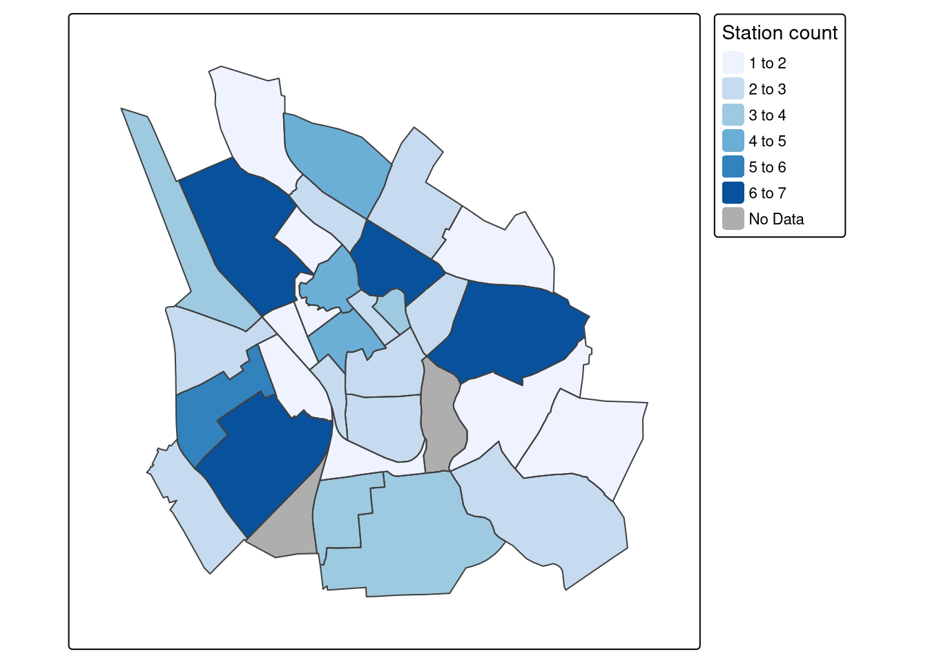
Let’s continue using our joined_dist_stations object and calculate the total bike count within each district. To achieve this, we can again use the group_by and summarise functions, but in this case focusing on the Rataste_arv variable, which represents the total number of bikes in each district.
# Total bike count within each district
bike_count <- joined_dist_stations %>%
group_by(NIMI) %>% # Group the data by district names (NIMI)
summarise(total_bikes = sum(Rataste_arv)) %>% # Calculate the sum of bikes
arrange(desc(total_bikes)) # Arrange the data in descending order
glimpse(bike_count)Rows: 33
Columns: 3
$ NIMI <chr> "Kesk-Annelinna", "Ülejõe", "Uus-Tammelinna", "Tähtvere", …
$ total_bikes <int> 153, 105, 87, 82, 81, 70, 63, 56, 51, 37, 34, 33, 31, 31, …
$ geom <MULTIPOLYGON [m]> MULTIPOLYGON (((661984.2 64..., MULTIPOLYGON …Let’s take a more detailed examination of the bike_count object using the summary function:
summary(bike_count) NIMI total_bikes geom
Length:33 Min. : 9.00 MULTIPOLYGON :33
Class :character 1st Qu.: 20.00 epsg:3301 : 0
Mode :character Median : 28.00 +proj=lcc ...: 0
Mean : 40.03
3rd Qu.: 54.75
Max. :153.00
NA's :3 The output indicates that the bike_count object contains three NAs, signifying three districts where shared bikes are unavailable. As per our earlier analysis, two of these districts lack sharing bikes. However, the third district appears to have a station but no actual shared bikes.
Let’s identify the districts where shared bikes are not available:
# Districts with no sharing bikes
no_bikes <- joined_dist_stations %>%
filter(is.na(Rataste_arv)) %>%
pull(NIMI)
no_bikes[1] "Kruusamäe" "Variku" "All-Karlova"Let’s plot the distribution of bikes in each district:
# Create tmap
tmap_mode("plot")ℹ tmap mode set to "plot".tm_shape(bike_count) +
tm_polygons(fill = "total_bikes",
fill.scale = tm_scale_intervals(
values = "brewer.reds", # Use the "Reds" color palette
label.na = 'No Data' # Label for areas with missing data
),
fill.legend = tm_legend(
title = "Bike count", # Set the title for the legend
position = tm_pos_out("right", "center"), # Place the legend outside of the map
frame = FALSE
)
) +
tm_borders() +
tm_layout(inner.margins = 0.1)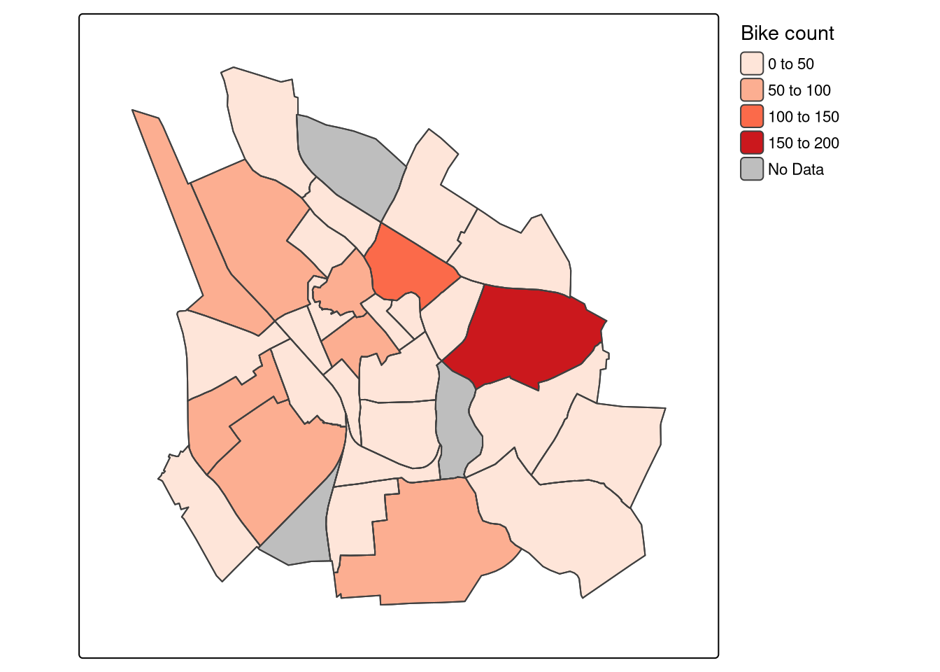
Exercise (15 minutes)
- Perform a spatial join to combine the ‘district’ and ‘shops’ datasets and identify the districts that contain NA values.
- Calculate the total number of shops per district and arrange the districts in descending order based on shop count.
- Identify the districts that contain NA values and have a single shop.
- Based on the outcome of the second task, visualize the result using tmap.
3.2. Non-overlapping joins
In some cases, two geographic datasets can display a significant geographical relationship even when they do not directly share spatial boundaries. Joining such non-overlapping spatial datasets becomes essential when we work with two datasets and intend to merge them, irrespective of whether they have common matching keys. A prominent example of this phenomenon can be observed in the stations and shops datasets. Visualizing these datasets reveals that they are often closely related but they do not touch or overlap.
tmap_mode("view")ℹ tmap mode set to "view".tm_shape(districts) +
tm_borders() +
tm_shape(stations) +
tm_symbols(fill = "red", size = 0.5) +
tm_shape(shops) +
tm_symbols(fill = "blue", size = 0.5) +
tm_layout(inner.margins = 0.1)Registered S3 method overwritten by 'jsonify':
method from
print.json jsonliteWe can check if there’s any contact or overlap between the geometries in the shops and stations datasets by using st_touches() function combined with any() function, resulting in either a TRUE or FALSE outcome.
# Transform 'shops' data to match the CRS of 'districts'
shops_3301 <- st_transform(shops, st_crs(districts))
# Check the overlap
any(st_touches(shops_3301, stations, sparse = FALSE))[1] FALSEThe above code returns a result of FALSE, indicating that there are no geometries in the shops_3301 object that touch or intersect with the geometries in the stations object.
The most straightforward approach for performing a non-overlapping join is using the binary predicate st_is_within_distance() and specifying a distance threshold.
# Create a logical vector indicating if shops are within 50 meters of stations
dist_50m <- st_is_within_distance(shops_3301, stations, dist = set_units(50, "m"))
dist_50mSparse geometry binary predicate list of length 4158, where the
predicate was `is_within_distance'
first 10 elements:
1: (empty)
2: (empty)
3: (empty)
4: (empty)
5: (empty)
6: (empty)
7: (empty)
8: (empty)
9: (empty)
10: (empty)The first 10 elements of the dist_50m object appear to be empty, meaning that there are no spatial relationships found within 50 m distance threshold for shops and stations datasets.
Let’s check for non-empty elements only within the dist_50m result. The next code will give you a summary of whether each element in the dist_50m list contains non-empty (i.e., TRUE) results.
# Check for non-empty elements (TRUE values) and create a summary
summary(lengths(dist_50m) > 0) Mode FALSE TRUE
logical 3840 318 The output reveals that there are 212 points (shops) in the target object shops_3301 within the threshold distance of stations. To retrieve these 212 shops, we will use the st_join() function with the dist parameter set to 50 meters.
# Perform the spatial join using st_is_within_distance and a 50m distance threshold
join_50m <- st_join(shops_3301, stations,
join = st_is_within_distance,
dist = 50)
#View(join_50m)Now let’s select shops that are within a 50-meter distance threshold:
# Select only the shops that are within a 50-meter distance of stations
shops_within_50m <- join_50m %>%
filter(!is.na(Asukoht))We can now create a visualization that displays shops located within a 50-meter radius of stations, along with both the shops and stations datasets:
tmap_mode("view")ℹ tmap mode set to "view".tm_shape(districts) +
tm_borders() +
tm_shape(stations) +
tm_symbols(fill = "red", size = 0.5) +
tm_shape(shops_3301) +
tm_symbols(fill = "blue", size = 0.5)+
tm_shape(shops_within_50m) +
tm_symbols(fill = "green", size = 0.5) +
tm_layout(inner.margins = 0.1)3.3. Buffers
Buffering geometries is one of the most common operations in GIS that involves creating a polygon representing the area within a specified distance around a geometry. Irrespective of the input geometry type, the result is always a polygon.
In R, buffering is straightforward using st_buffer() function from the sf package. The function takes an sf object as input, which we want to create buffers around, and the distance of the buffer specified in a unit of length, such as meters.
In this lesson, we will use the stations data to generate a buffer with a radius of 200 meters around each station.
#Check the unit of `stations` object
st_crs(stations)$units [1] "m"# Generate 200 m buffer
stations_buffer_200 <- st_buffer(stations, dist = 200) The result should appear like this, where the red color indicates the buffered stations, and the original stations are displayed in black:
tmap_mode("view")ℹ tmap mode set to "view".tm_shape(districts) +
tm_borders() +
tm_shape(stations_buffer_200) +
tm_symbols(fill = "red", size = 1)+
tm_shape(stations) +
tm_symbols(fill = "black", size = 0.1) +
tm_layout(inner.margins = 0.1)Now, let’s work with the stations_buffer_200 object and conduct a query to identify shops located within the buffered area. To do this, we’ll begin by executing a spatial join between the shops_3301 and stations_buffer_200 objects.
# Perform a spatial join to select shops within the buffered zone
shops_within_buffer <- st_join(shops_3301, stations_buffer_200, left = FALSE)
glimpse(shops_within_buffer)Rows: 4,068
Columns: 10
$ osm_id <chr> "266921299", "322906403", "322906403", "326236651", "33080…
$ OBJECTID <dbl> 6859, 6820, 6857, 6862, 6811, 6876, 6811, 6876, 6835, 6820…
$ Rataste_arv <int> 10, 15, 20, 16, 18, 12, 18, 12, 11, 15, 16, 12, 12, 12, 12…
$ Asukoht <chr> "51 Lõunakeskus", "12 Roosi", "49 Raatuse", "54 Veeriku", …
$ Markus <chr> NA, NA, NA, NA, NA, NA, NA, NA, NA, NA, NA, NA, NA, NA, NA…
$ Omanik <int> 3, 3, 3, 3, 3, 3, 3, 3, 3, 3, 3, 3, 3, 3, 3, 3, 3, 3, 3, 3…
$ Staatus <int> 1, 1, 1, 1, 1, 1, 1, 1, 1, 1, 1, 1, 1, 1, 1, 1, 1, 1, 1, 1…
$ P_aasta <int> 2019, 2019, 2019, 2019, 2019, 2019, 2019, 2019, 2019, 2019…
$ Linnaosa <int> 10, 17, 17, 16, 1, 1, 1, 1, 14, 17, 17, 1, 1, 1, 1, 1, 14,…
$ geom <POINT [m]> POINT (656645.8 6471739), POINT (659668.7 6474583), …Make sure that you use the argument left = FALSE, which ensures that only shops that intersect with buffered stations are retained.
Let’s create a visualization that displays the shops located within the buffered zone, along with the buffered stations and the entire shops dataset.
# Create the map
tmap_mode("view")ℹ tmap mode set to "view".tm_shape(districts) +
tm_borders() +
tm_shape(stations_buffer_200) +
tm_symbols(fill = "red", size = 0.5) +
tm_shape(shops_3301) +
tm_symbols(fill = "blue", size = 0.5) +
tm_shape(shops_within_buffer) +
tm_symbols(fill = "#00FF00", size = 0.5) +
tm_layout(inner.margins = 0.1)Exercise (10 minutes)
Generate a 500-meter buffer around the Emajõgi river and identify the shops located within this buffer zone.
3.4. Distance
The distance between any two spatial points can be computed using both of its coordinate points. In R, the st_distance() function from sf package can be used to compute the distance between the specified set of points. It returns a numeric matrix containing the distances between the specified geometries.
The following code allows us to find the distance between two bike stations, Vanemuise park and Raatuse. We start by selecting the target stations and then use st_distance() to compute the distance.
# Subsets the target stations
Vanemuise <- stations[stations$Asukoht == "Vanemuise park", ]
Raatuse <- stations[stations$Asukoht == "49 Raatuse", ]
# Calculate distance
distance <- st_distance(Vanemuise, Raatuse)
# Print the calculated distance
distanceUnits: [m]
[,1]
[1,] 1406.328Great! We’ve successfully calculated the distance between the Vanemuise and Raatuse bike stations, which is around 1406 meters. Now, let’s create a line connecting these stations.
# Coordinates of the Vanemuise and Raatuse stations
Vanemuise[c("lon", "lat")] <- st_coordinates(Vanemuise) # X and Y coords. from the Geom column in stations object
Raatuse[c("lon", "lat")] <- st_coordinates(Raatuse)
# Convert to data frames and combine them into a single data frame
Vanemuise_df <- data.frame(lon = Vanemuise$lon, lat = Vanemuise$lat)
Raatuse_df <- data.frame(lon = Raatuse$lon, lat = Raatuse$lat)
pts <- rbind(Vanemuise_df, Raatuse_df)
# Convert the data frame to sf format and set projection to EPSG:3301
points_sf <- st_as_sf(pts, coords = c("lon", "lat"))
points_sf <- st_set_crs(points_sf, 3301)
# Convert points to a line and set projection to EPSG:3301
sf_lines <- points_sf %>%
st_union() %>%
st_cast("LINESTRING")
sf_lines <- st_set_crs(sf_lines, 3301)Plot the results:
# Plot
tmap_mode("view")ℹ tmap mode set to "view".tm_shape(districts) +
tm_borders() +
tm_shape(stations) +
tm_symbols(fill = "blue", size = 0.5) +
tm_shape(points_sf) +
tm_dots(fill = "green", size = 0.4) +
tm_shape(sf_lines) +
tm_lines(col = "red", lwd = 2) +
tm_layout(inner.margins = 0.1)Next, we’ll compute the Euclidean distance between all the stations. The Euclidean distance represents the straight-line distance between any two points, in our case, between two stations. The code below calculates Euclidean distances between all pairs of stations (totaling 101 stations) and store the result in the dist_matrix.
# Calculate the distance matrix
dist_matrix <- st_distance(stations, method = "euclidean")
# Print the distance matrix
#dist_matrixThe elements in the dist_matrix correspond to pairs of individual stations, with the value at the intersection of a specific row and column denoting the distance between the stations associated with those row and column positions.
Let’s check the longest and mean distances between stations:
max(dist_matrix)18918.99 [m]mean(dist_matrix)3643.874 [m]We can generate a histogram to visualize all the distances and gain a holistic understanding of their distribution.
# Create a histogram of the distances
hist(as.vector(dist_matrix),
main = "Distance Histogram",
xlab = "Distance (m)",
ylab = "Frequency",
col = "lightblue")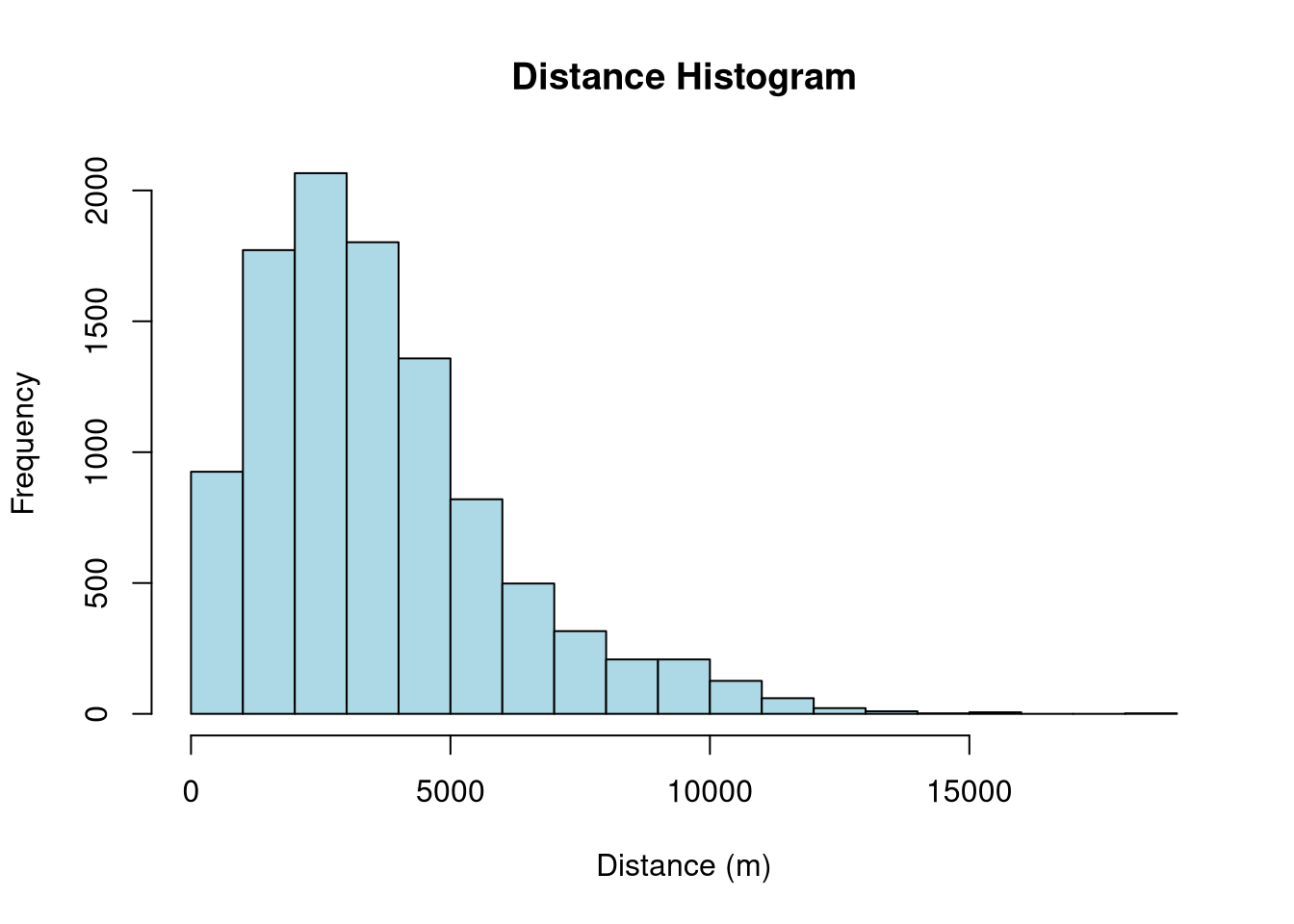
The histogram of bike station distances reveals that the most frequent distance between stations is 2000m, indicating a concentration of stations at this specific distance in the dataset.
3.5. Union
Geometric union refers to the process of combining or merging multiple geometric features, such as spatial polygons, into a single and unified geometry. In R, the process of performing geometric unions can be achieved using the st_union() function available in the sf package.
In this lesson, we will illustrate geometric unions through the process of merging Estonia’s individual municipalities to form a new geometric entity that represents the national boundary of Estonia.
Download Estonian municipalities data using this link and save it in your current working directory (R_03 folder).
# Import municipalities data
municip <- st_read("municipalities.gpkg")Reading layer `municipalities' from data source
`/workdir/R_03/municipalities.gpkg' using driver `GPKG'
Simple feature collection with 79 features and 5 fields
Geometry type: MULTIPOLYGON
Dimension: XY
Bounding box: xmin: 369033.8 ymin: 6377141 xmax: 739152.8 ymax: 6634019
Projected CRS: Estonian Coordinate System of 1997glimpse(municip)Rows: 79
Columns: 6
$ ONIMI <chr> "Saaremaa vald", "Tallinn", "Anija vald", "Ruhnu vald", "Vormsi …
$ OKOOD <chr> "0714", "0784", "0141", "0689", "0907", "0255", "0245", "0198", …
$ MNIMI <chr> "Saare maakond", "Harju maakond", "Harju maakond", "Saare maakon…
$ MKOOD <chr> "0074", "0037", "0037", "0074", "0056", "0052", "0037", "0037", …
$ TYYP <chr> "1", "4", "1", "1", "1", "1", "1", "1", "1", "1", "1", "1", "1",…
$ geom <MULTIPOLYGON [m]> MULTIPOLYGON (((383803.2 64..., MULTIPOLYGON (((542…Now, let’s unite the boundaries of all municipalities by employing the st_union() function and generate a new object of the sfc class:
# Merge all geometries into one
est_union <- sf::st_union(municip)
class(est_union)[1] "sfc_MULTIPOLYGON" "sfc" Let’s visualize it:
# Plot
tmap_mode("plot")ℹ tmap mode set to "plot".tm_shape(est_union)+
tm_borders()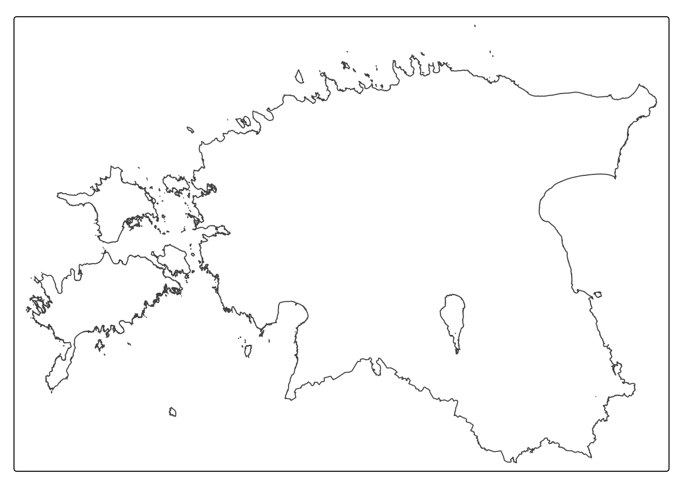
We can also merge all municipalities within a specific county to create a new object representing Estonia’s 15 counties. Behind the scenes, group_by() and summarize() functions combine the geometries using st_union().
The following code combines individual municipalities within a specific county from the municip object and generates a new object called est_counties containing the integrated polygons.
# Create a new object named est_counties
est_counties <- municip %>%
group_by(MNIMI) %>%
summarize() %>%
ungroup() Our est_counties object now comprises unified polygons that represent 15 counties of Estonia.
Let’s visualize it.
# Remove the word "maakond" from all counties
est_counties$MNIMI <- sub(" maakond$", "", est_counties$MNIMI)
# The sub function is used to perform a substitution operation on the values in the MNIMI column.
# Plot
tmap_mode("plot")ℹ tmap mode set to "plot".tm_shape(est_counties)+
tm_polygons(fill = "MNIMI",
fill.legend = tm_legend(
title = "County",
position = tm_pos_out("right", "center") # Place the legend outside of the map
),
col_alpha = 0.2, # Adjust the transparency of the borders between 0 and 1; 0 → Fully transparent and 1 → Fully opaque
frame = FALSE
) +
tm_layout(inner.margins = 0.1) [tm_polygons()] Argument `frame` unknown.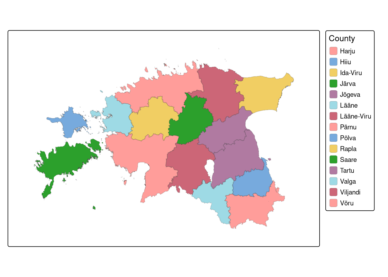
3.6. Clipping
Clipping vector data refers to creating a new layer that contains only the data within a specified geographical extent or boundary. Although the sf package does not offer a direct clip function, the st_intersection() can achieve the same goal. However, it is important to note that intersection creates output features that retain the attributes of all input features.
Let’s extract the Tartu district from the est_union object we created earlier.
# Transform 'est_union' to match the CRS of 'districts'
est_union <- st_transform(est_union, st_crs(districts))
# Check if the CRS of 'est_union' and 'districts' are identical
identical(st_crs(est_union), st_crs(districts))[1] TRUE# Perform the intersection operation to obtain 'clipped_dist'
clipped_dist <- st_intersection(est_union, districts)Let’s plot the clipped object on top of the map of Estonia:
# Create the thematic map
tm_shape(est_union) +
tm_polygons(fill = "grey") +
tm_shape(st_union(clipped_dist))+
tm_polygons(fill = "red") 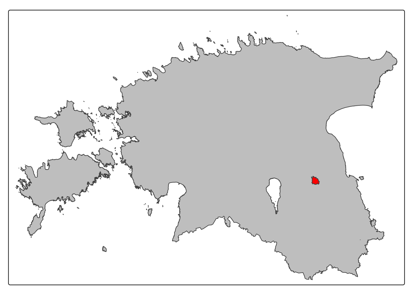
Exercise (10 minutes)
Clip Emajõgi river within the geographical boundary of the Tartu district.